Linear regression
Applied Statistics for Life Sciences
PREVEND data
Ruff Figural Fluency Test (RFFT) is a cognitive assessment.
- measures nonverbal fluency and executive cognitive function
- scale: 0 (worst) to 175 (best)
| casenr | age | rfft |
|---|---|---|
| 126 | 37 | 136 |
| 33 | 36 | 80 |
| 145 | 37 | 102 |
| 146 | 37 | 85 |

Question of interest:
How much does cognitive ability as measured by RFFT decline with age on average?
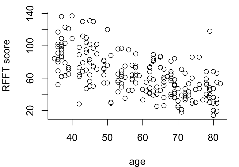
PREVEND data
Ruff Figural Fluency Test (RFFT) is a cognitive assessment.
- measures nonverbal fluency and executive cognitive function
- scale: 0 (worst) to 175 (best)
| casenr | age | rfft |
|---|---|---|
| 126 | 37 | 136 |
| 33 | 36 | 80 |
| 145 | 37 | 102 |
| 146 | 37 | 85 |
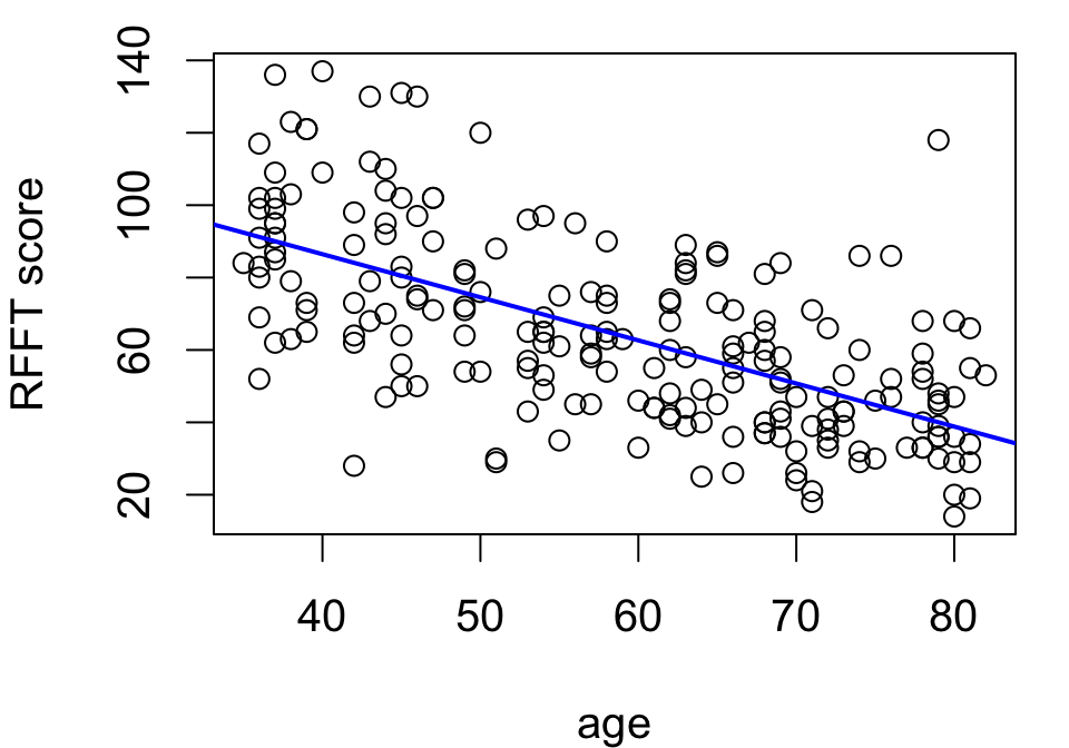
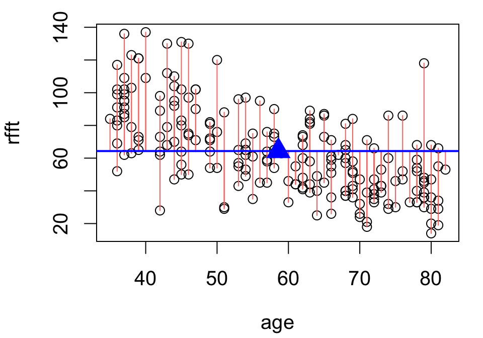
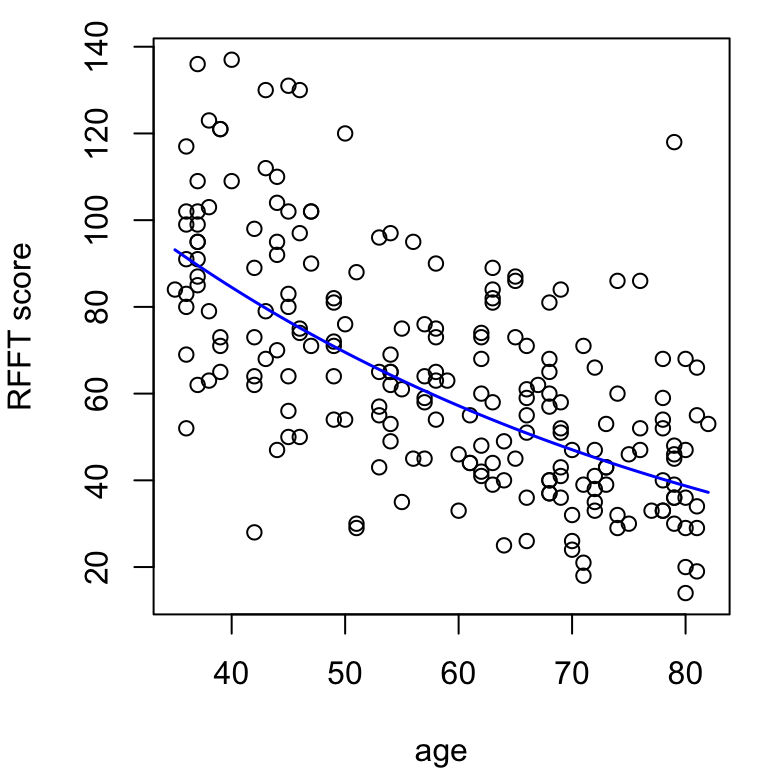
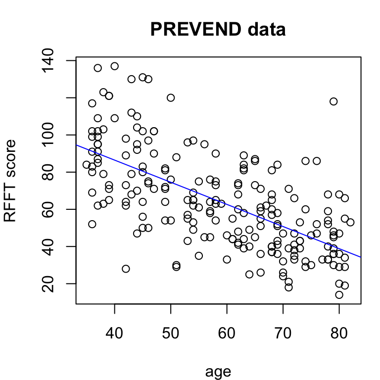
A straight line seems to describe the RFFT-age relationship well enough.
This suggests a model:
- mean RFFT is a linear function of age
- remaining variation in RFFT is random
Lines
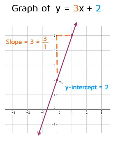
The equation of a line in slope-intercept form is:
\[ y = ax + b \]
\(a\) is the slope (rise over run) and \(b\) is the intercept:
- the line crosses the \(y\) axis at \(b\)
- \(y\) changes by \(a\) per unit increment in \(x\)
There is exactly one line through any two points.
Linear trends in data
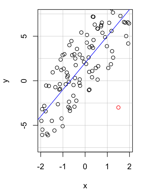
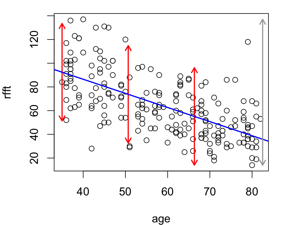
We say a set of data points \((x_i, y_i)\) exhibit a linear trend if the points fall “near” a line.
Some things to keep in mind:
- real data will never fall exactly on a line
- there may be outliers (e.g., red point at right)
- points could be pretty far spread out and still exhibit a linear trend
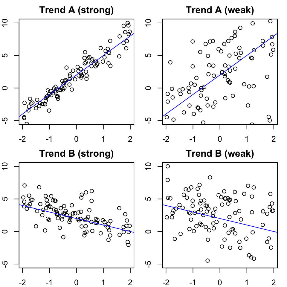
Linear trends in data
We can articulate two properties of linear trends:
- direction: positive (A) or negative (B)
- strength: concentration about line
Note that trends in each row are identical.
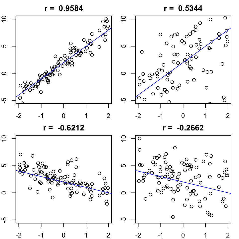
Correlation
Correlation is a signed measure of strength of linear relationship.
\[ r = \frac{\sum_i (x_i - \bar{x})(y_i - \bar{y})}{s_x \times s_y} \]
When data points are far from the mean at the same time in the same direction, the magnitude will be larger.
- sign indicates direction of relationship
- magnitude indicates strength (always between -1 and 1)
Common mistake: strength \(\neq\) slope.
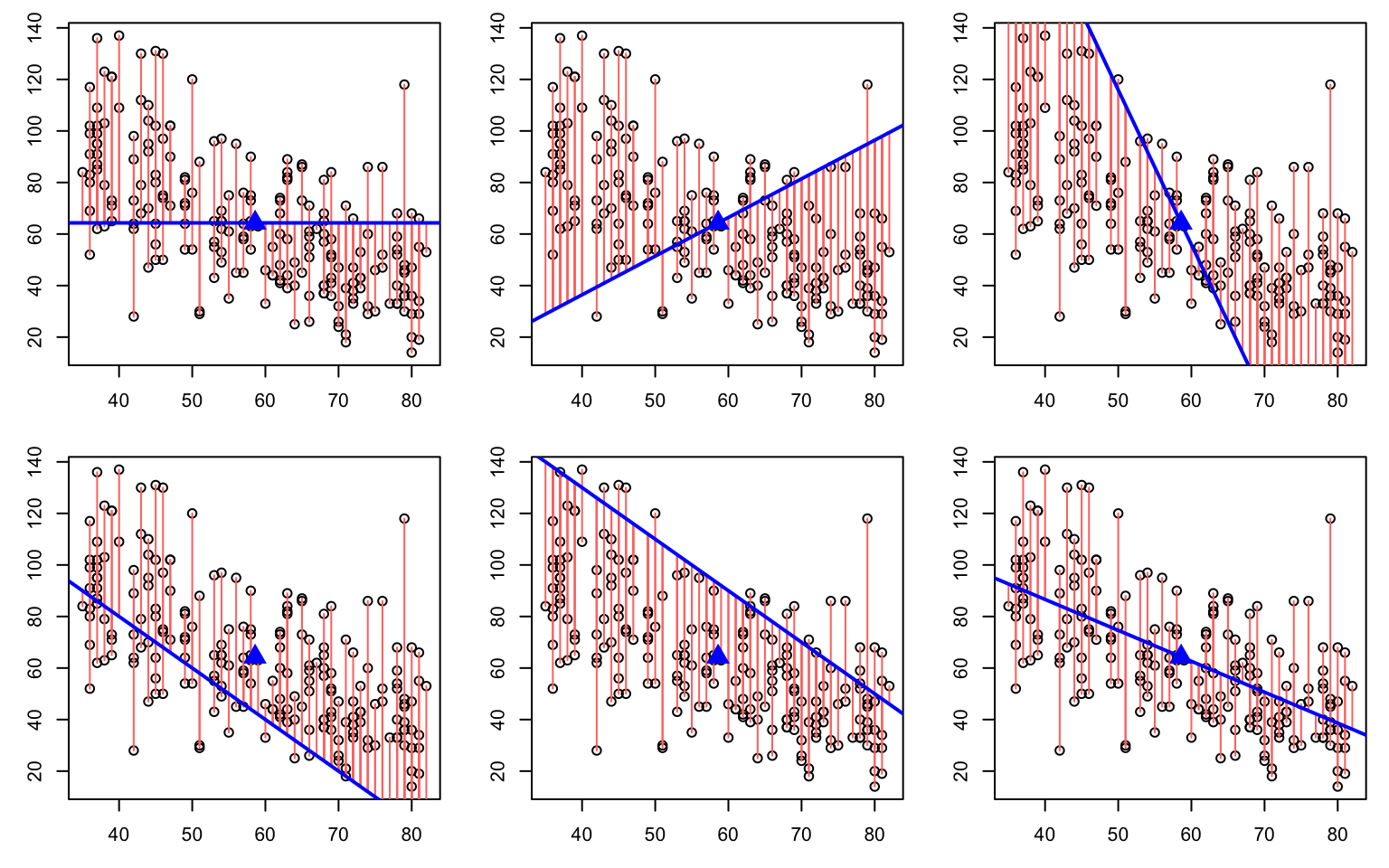
Fitting lines to data
Fitting lines to data
Most of these are bad. Some are worse than others. How might one measure this?
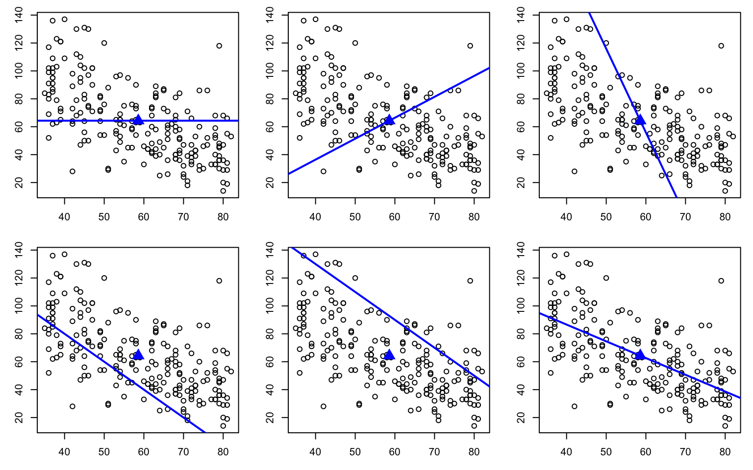
Fitting lines to data
Hint: consider the residuals – distances from the line to each point.
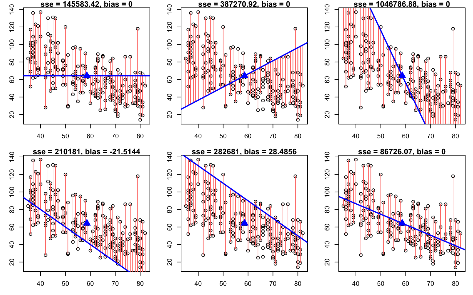
Measuring quality of fit
Residuals are the distances to each point: \[ \textcolor{red}{e_i} = y_i - \textcolor{blue}{\hat{y}_i} \]
Quality of fit can be measured by:
- [bias] average error \(-\frac{1}{n}\sum_i \textcolor{red}{e_i}\)
- [SSE] total (squared) error \(\sum_i \textcolor{red}{e_i}^2\)
Measuring quality of fit
Now consider what the bias and SSE (total squared error) capture.
Least squares line
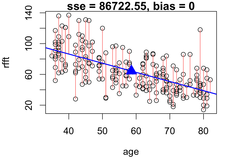
The line with no bias and minimal total error is called the least squares line:
\[ \text{RFFT} = 134.098 - 1.191 \times \text{age} \]
With each year of age, RFFT decreases by 1.191 points on average.
The least squares line has an analytic solution:
\[ \begin{align} \text{slope}: \quad-1.191 &= \text{cor}(\text{age}, \text{RFFT})\times\frac{SD(\text{RFFT})}{SD(\text{age})} \\ \text{intercept}: \quad134.098 &= \text{mean}(\text{RFFT}) - (-1.191)\times\text{mean}(\text{age}) \end{align} \]
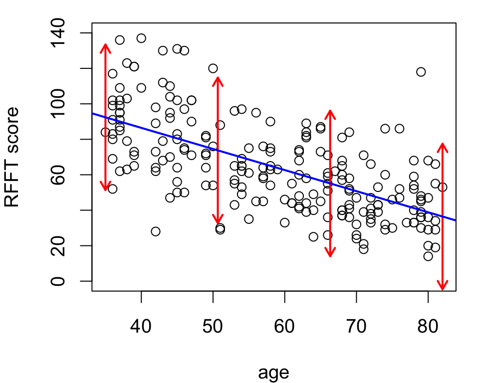
Error variability and model fit
The residual standard deviation provides an estimate of error variability:
\[\textcolor{\red}{\hat{\sigma}} = \sqrt{\frac{1}{n - 2} \sum_i e_i^2} \qquad\text{(estimated error variability)}\]
The proportion of variability explained by the model is: \[ R^2 = 1 - \frac{(n - 2)\textcolor{red}{\hat{\sigma}^2}}{(n - 1)\textcolor{darkgrey}{s_y^2}} \quad\left(1 - \frac{\text{error variability}}{\text{total variability}}\right) \]
Age explains 40.43% of variability in RFFT.
Model specification
Is the relationship actually linear?
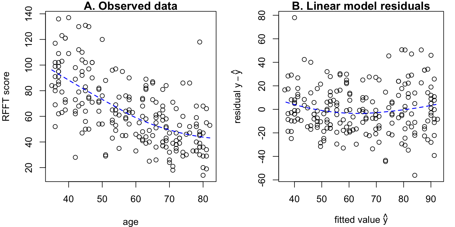
Two ways to check:
- Inspect observed data for nonlinear trend
- Inspect model residuals for “patterns”
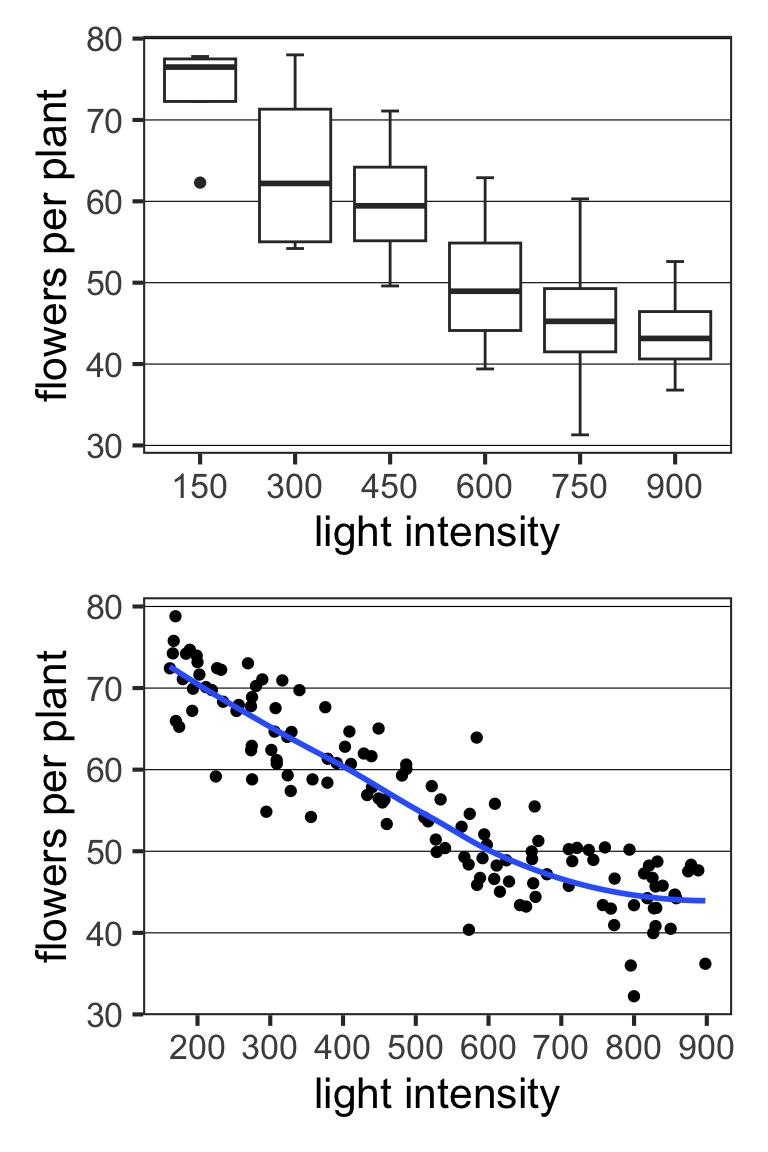
Local smoothing is shown in blue.
The linear model is a fine approximation here – the curvature is very minor – but let’s consider an alternative model specification as a thought exercise.
An alternative model
\[ \log(\text{RFFT}) = \beta_0 + \beta_1\times\text{age} + \epsilon \]
The model now implies that the mean RFFT score is a nonlinear function of age:
\[ \text{RFFT} \propto e^{\beta_1\text{age}} \]
And we can still fit it using least squares:
Linear models can be used to capture more than just linear relationships!
Kleiber’s law
Kleiber’s law refers to the relationship between metabolic rate and body mass.
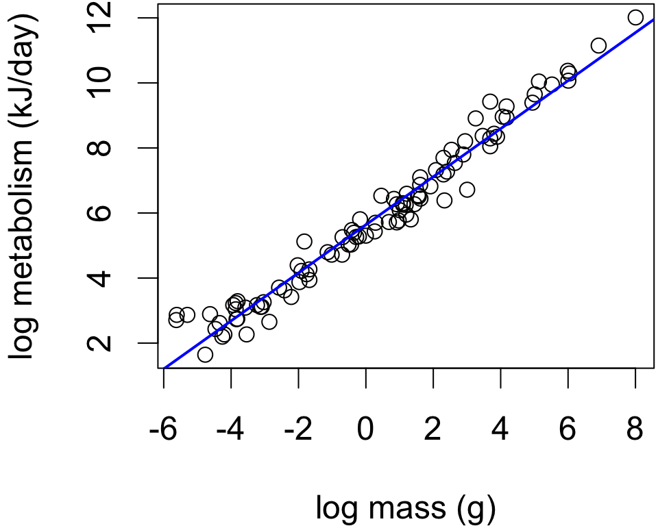
We can estimate it via the SLR model: \[ \log(\text{metabolism}) = \beta_0 + \beta_1 \log(\text{mass}) + \epsilon \]
Fitted model: \[ \log(\text{metabolism}) = 5.64 + 0.74 \times \log(\text{mass}) \]
Review
How much does RFFT decline with age?
Simple linear regression (SLR) model: \[ \text{RFFT} = \beta_0 + \beta_1\text{age} + \epsilon \]
Call:
lm(formula = rfft ~ age, data = prevend)

Coefficients:
(Intercept)          age
134.098 -1.191 Interpretation:
With each additional year of age, mean RFFT score decreases by an estimated 1.191 points.
Review
The residual standard deviation is an estimate of the unexplained variation in RFFT.
More unexplained variation entails more sampling variability in the model fit.
Inference for the slope parameter
If the errors are symmetric and unimodal, then the sampling distribution of \[ T = \frac{\hat{\beta}_1 - \beta_1}{SE(\beta_1)} \] is well-approximated by a \(t_{n - 2}\) model.
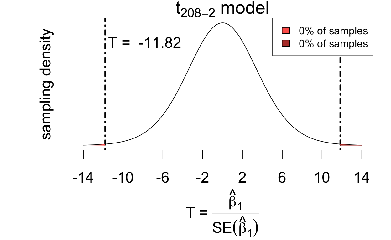
Significance test: \(\begin{cases} H_0: \beta_1 = 0 \\ H_A: \beta_1 \neq 0 \end{cases}\)
Confidence interval: \(\hat{\beta}_1 \pm c\times SE\left(\hat{\beta}_1\right)\)
\(P(T > |T_\text{obs}|) \approx 0\): evidence of an association (true slope is not zero)
confidence interval using \(t_{206}\) critical value: (-1.389, -0.992)
Inference for the intercept is analogous, but not very common.
Prediction in SLR
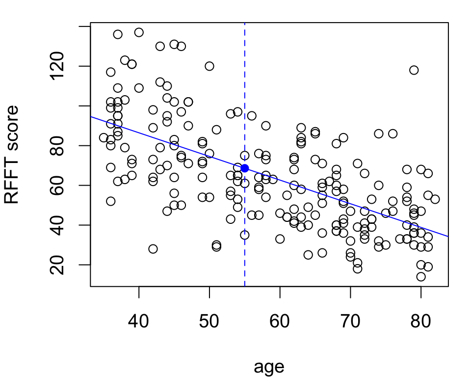
Intervals for the mean
There are two possible ways to interpret model predictions:
- The estimated mean RFFT score for 55-year-olds is 68.6
- The predicted value of RFFT for a specific 55-year-old individual is 68.6
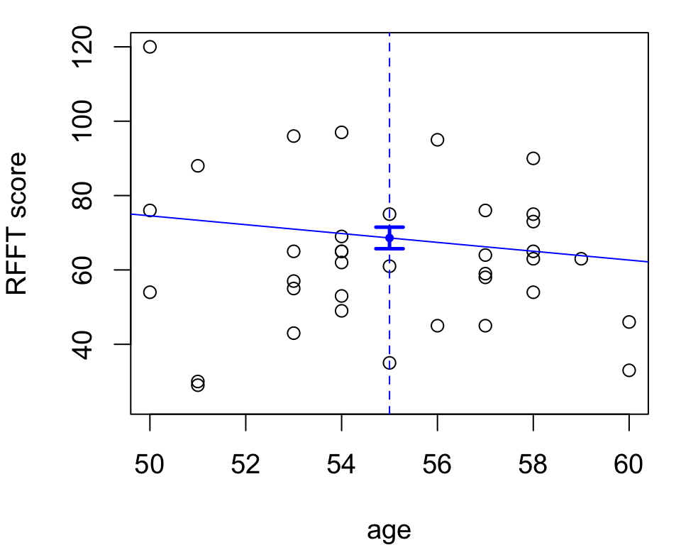
With 95% confidence, the mean RFFT score among 55-year-olds is estimated to be between 65.71 and 71.50 points.
Intervals for predicted values
There are two possible ways to interpret model predictions:
- The estimated mean RFFT score for 55-year-olds is 68.6
- The predicted value of RFFT for a specific 55-year-old individual is 68.6
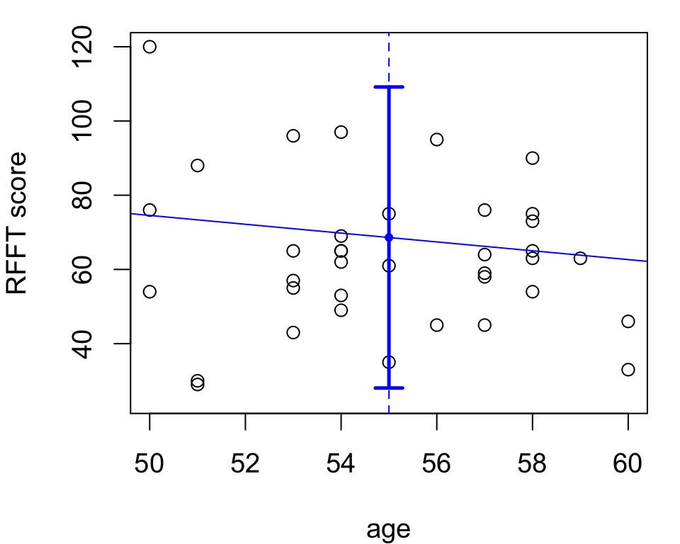
With 95% confidence, the RFFT score for an individual 55 year old is estimated to be between 28.05 and 109.16 points.
Uncertainty bands
Pointwise intervals shown along the line provide a visual of the model uncertainty.
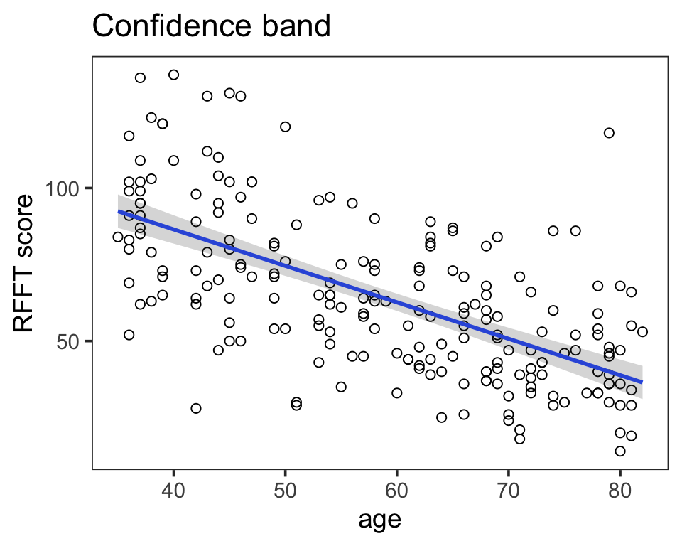
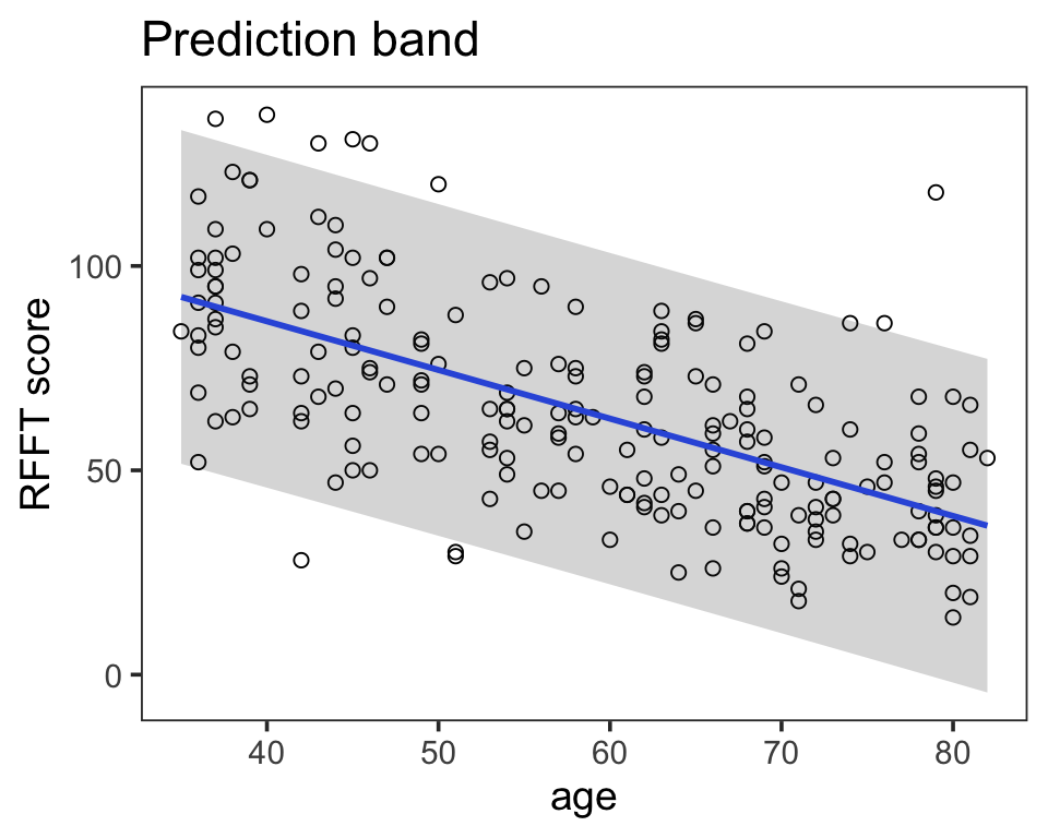
Why the difference? Individual observations are more variable than averages.
Kleiber’s law
Call:
lm(formula = log.metab ~ log.mass, data = kleiber)

Residuals:
     Min       1Q   Median       3Q      Max
-1.14216 -0.26466 -0.04889  0.25308  1.37616

Coefficients:
            Estimate Std. Error t value Pr(>|t|)
(Intercept)  5.63833    0.04709  119.73   <2e-16 ***
log.mass     0.73874    0.01462   50.53   <2e-16 ***
---
Signif. codes:  0 '***' 0.001 '**' 0.01 '*' 0.05 '.' 0.1 ' ' 1

Residual standard error: 0.4572 on 93 degrees of freedom
Multiple R-squared:  0.9649,    Adjusted R-squared:  0.9645
F-statistic:  2553 on 1 and 93 DF,  p-value: < 2.2e-16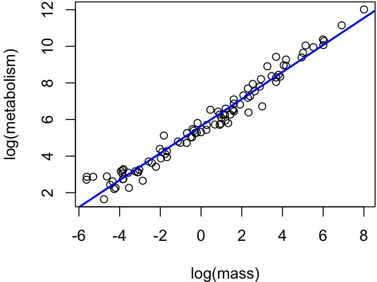
- \(\hat{\beta}_0 = 5.638, \hat{\beta}_1 = 0.739, \hat{\sigma} = 0.457\)
There is a significant association between body mass and metabolism (p < 0.0001): body mass explains 96.49% of variation in metabolism; with 95% confidence, a unit increment in log mass is associated with an estimated increase in mean log metabolism between 0.7097 and 0.7678.
Kleiber’s law
How much energy do we consume on a daily basis?
Conversions:
- 110lb \(\approx\) 50kg
- 180lb \(\approx\) 80kg
- 1 kJ \(\approx\) 0.239 kcal
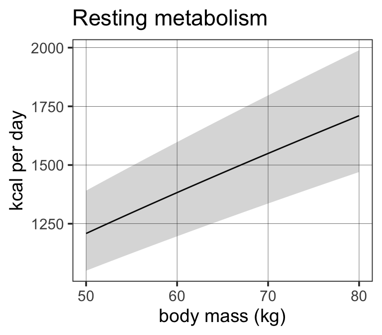
Using the SLR model, estimated resting energy consumption is:
\[ \hat{y} = 281\times\text{mass}^{0.74} \]
Left, prediction curve with 95% confidence interval.
Kleiber’s law
How much energy do you consume on a daily basis?
Conversions:
- 110lb \(\approx\) 50kg
- 180lb \(\approx\) 80kg
- 1 kJ \(\approx\) 0.239 kcal
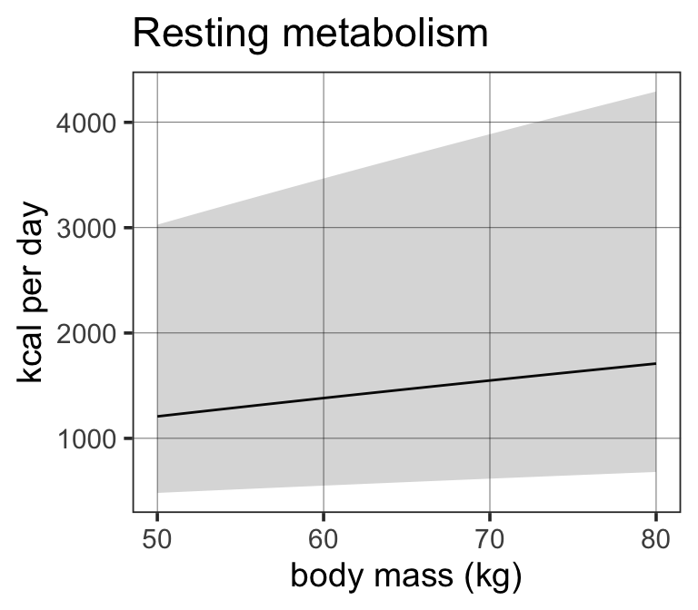
Using the SLR model, estimated resting energy consumption is:
\[ \hat{y} = 281\times\text{mass}^{0.74} \]
Left, prediction curve with 95% prediction interval.
Hubble constant
The Hubble constant \(H\) relates a galaxy’s relative distance and velocity as \(H = \frac{v}{d}\).
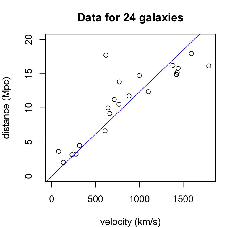
Least squares estimate of \(\beta = \frac{1}{H}\):
\[ \hat{\beta} = 0.0123 \]
90% CI for the age of the universe:
# interval for age of universe in bn yr
km.mpc <- 3.09e19
yr.sec <- 1/(60*60*24*365)
confint(fit, level = 0.9)*km.mpc*yr.sec/1e9
5 % 95 %
velocity 10.98235 13.12108With 90% confidence, the universe is estimated to be between 10.98 and 13.12 billion years old.