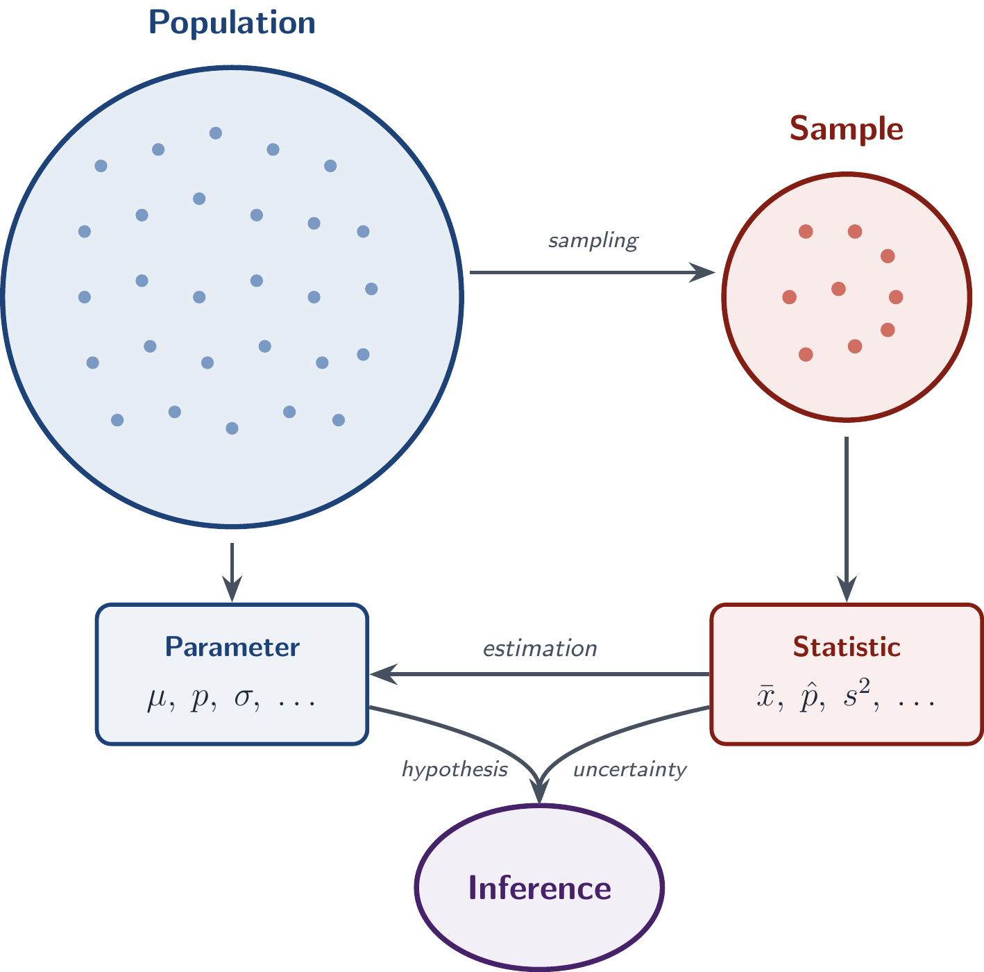
Course recap

Applied Statistics for Life Sciences

Big picture

In STAT218 we cover statistical inference for:

  • means and proportions
  • with/without grouping or covariates
  • for independent data

But the basic framework generalizes quite broadly.

One framework, many methods

Every method in this course follows the same logical template:

  1. Parameter — the unknown population quantity of interest
  2. Statistic — a point estimate computed from the sample
  3. Standard error — quantifies sampling variability of the statistic
  4. Test statistic — how far is the estimate from the null value, in SE units?
  5. p-value — probability of a result this extreme if \(H_0\) were true
  6. Confidence interval — plausible range of values for the parameter

What changes from method to method is what fills each slot — the logic stays the same.

Reporting results

Almost every result in this course can be reported in one of two forms:

Test result:

The data provide [evidence / no evidence] that [claim about parameter].

Interval estimate:

With 95% confidence, [parameter] is estimated to be between [lower] and [upper].

Inference for one mean

The method

Data: \(n\) measurements of a continuous variable.

Parameter: population mean \(\mu\)

Hypotheses: \(\quad\begin{cases} H_0: \mu = \mu_0 \\ H_A: \mu \neq \mu_0 \quad\text{(or } <, > \text{)} \end{cases}\)

Test statistic: \(\quad T = \dfrac{\bar{x} - \mu_0}{SE(\bar{x})} \quad\text{where}\quad SE(\bar{x}) = \dfrac{s_x}{\sqrt{n}}\)

Sampling distribution: \(\quad t_{n - 1}\) model

Confidence interval: \(\quad \bar{x} \pm c \times SE(\bar{x})\)

Assumptions: observations are independent; underlying distribution is approximately normal (robust for large \(n\)).

Example: body temperatures

Is the true mean body temperature actually 98.6°F?
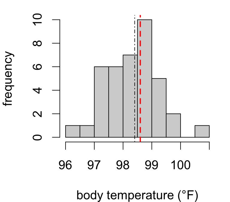
t.test(temps$body.temp, mu = 98.6)

    One Sample t-test

data:  temps$body.temp
t = -1.3283, df = 38, p-value = 0.192
alternative hypothesis: true mean is not equal to 98.6
95 percent confidence interval:
 98.10813 98.70213
sample estimates:
mean of x 
 98.40513 

The data provide evidence that mean body temperature differs from 98.6°F (T = -2.24 on 129 degrees of freedom, p = 0.027). With 95% confidence, the mean is estimated to be between 98.12 and 98.57°F.

Example: hours of sleep

Do U.S. adults sleep an average of 8 hours per night? (NHANES data)
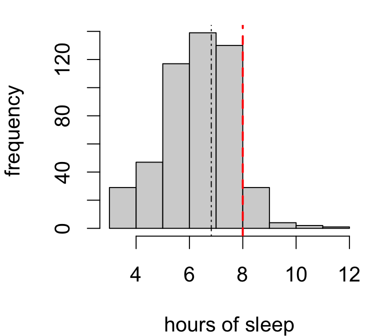
t.test(nhanes$sleephrsnight, mu = 8)

    One Sample t-test

data:  nhanes$sleephrsnight
t = -19.327, df = 497, p-value < 2.2e-16
alternative hypothesis: true mean is not equal to 8
95 percent confidence interval:
 6.699248 6.939307
sample estimates:
mean of x 
 6.819277 

The data provide evidence that the average U.S. adult does not sleep 8 hours per night (T = -42.53 on 3178 degrees of freedom, p < 0.0001). With 95% confidence, the mean nightly hours of sleep among U.S. adults is estimated to be between 6.91 and 7.01 hours.

Inference for two means

The method

Data: measurements of a continuous variable from two groups (paired or independent).

Testing a mean difference (paired data): inference on \(\delta = \mu_\text{before} - \mu_\text{after}\) or similar.

  • compute differences \(d_i\) and apply one-sample inference

Testing a difference in means (independent samples): inference on \(\mu_1 - \mu_2\).

Test statistic: \(\quad T = \dfrac{\bar{x} - \bar{y}}{SE(\bar{x} - \bar{y})} \quad\text{where}\quad SE = \sqrt{\dfrac{s_x^2}{n_x} + \dfrac{s_y^2}{n_y}}\)

Sampling distribution: \(\quad t_\nu\) model

Confidence interval: \(\quad (\bar{x} - \bar{y}) \pm c \times SE(\bar{x} - \bar{y})\)

Example: desired weight

Does the average U.S. adult wish to lose weight?
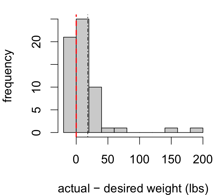
weight.diffs <- brfss$weight - brfss$wtdesire
t.test(weight.diffs, mu = 0, 
       alternative = 'greater')

    One Sample t-test

data:  weight.diffs
t = 4.2172, df = 59, p-value = 4.311e-05
alternative hypothesis: true mean is greater than 0
95 percent confidence interval:
 10.99824      Inf
sample estimates:
mean of x 
 18.21667 

The data provide evidence that the average U.S. adult’s actual weight exceeds their desired weight (T = 4.2172 on 59 degrees of freedom, p < 0.0001).

Example: finch beak depth

Did beak depth increase after the 1977 drought on Daphne Major?
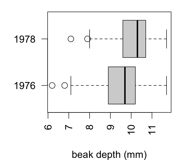
t.test(depth ~ year, data = finch, 
       alternative = 'less')

    Welch Two Sample t-test

data:  depth by year
t = -4.5833, df = 172.98, p-value = 4.37e-06
alternative hypothesis: true difference in means between group 1976 and group 1978 is less than 0
95 percent confidence interval:
      -Inf -0.427321
sample estimates:
mean in group 1976 mean in group 1978 
          9.469663          10.138202 

The data provide evidence that mean beak depth increased following the drought (T = -4.57 on 111.79 degrees of freedom, p < 0.0001).

Inference for many means

ANOVA

Data: measurements of a continuous variable across \(k > 2\) groups.

Parameter: group means \(\mu_1, \dots, \mu_k\)

Hypotheses: \(\quad\begin{cases} H_0: \mu_1 = \mu_2 = \cdots = \mu_k \\ H_A: \text{at least two means differ} \end{cases}\)

Test statistic: \(\quad F = \dfrac{MSG}{MSE} \quad \left(\frac{\text{group variation}}{\text{individual variation}}\right)\)

Sampling distribution: \(\quad F_{k - 1,\; n - k}\) model

Effect size: \(\quad \eta^2 = \dfrac{SSG}{SSG + SST} \quad \left(\frac{\text{group variation}}{\text{total variation}}\right)\)

Post-hoc: pairwise contrasts \(\mu_i - \mu_j\) with multiple testing adjustment.

ANOVA table

Source degrees of freedom Sum of squares Mean square F statistic p-value
Group \(k - 1\) SSG \(MSG = \frac{SSG}{k - 1}\) \(\frac{MSG}{MSE}\) \(P(F > F_\text{obs})\)
Error \(n - k\) SSE \(MSE = \frac{SSE}{n - k}\)
  • the SS terms are ‘raw’ measures of variability from each source
  • the MS terms are adjusted for the amount of data and number of parameters

Formally, the ANOVA model says \[\underbrace{(n - 1)S^2}_{SST} = SSG + SSE\]

Example: diet and longevity

Does caloric restriction affect mean lifespan in mice?
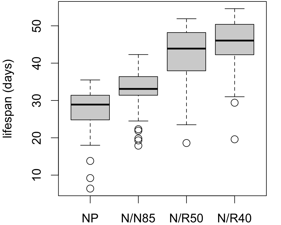
fit <- aov(lifetime ~ diet, data = longevity)
summary(fit)
             Df Sum Sq Mean Sq F value Pr(>F)    
diet          3  11426    3809   87.41 <2e-16 ***
Residuals   233  10152      44                   
---
Signif. codes:  0 '***' 0.001 '**' 0.01 '*' 0.05 '.' 0.1 ' ' 1
eta_squared(fit, partial = FALSE, 
            alternative = 'two.sided')
# Effect Size for ANOVA (Type I)

Parameter | Eta2 |       95% CI
-------------------------------
diet      | 0.53 | [0.44, 0.60]

The data provide evidence that diet restriction has an effect on mean lifetime among mice (F = 87.41 on 3 and 233 degrees of freedom, p < 0.0001). With 95% confidence, the proportion of variation in lifespan explained by diet is estimated to be between 44% and 60%.

Post-hoc comparisons

Which diets differ? Pairwise contrasts with Bonferroni correction:

emmeans(fit, ~ diet) |>
  contrast('pairwise') |>
  test(adjust = 'bonferroni')
 contrast          estimate   SE  df t.ratio p.value
 NP - (N/N85)         -5.29 1.29 233  -4.113  0.0003
 NP - (N/R50)        -14.90 1.23 233 -12.150 <0.0001
 NP - (N/R40)        -17.71 1.27 233 -13.938 <0.0001
 (N/N85) - (N/R50)    -9.61 1.17 233  -8.183 <0.0001
 (N/N85) - (N/R40)   -12.43 1.22 233 -10.177 <0.0001
 (N/R50) - (N/R40)    -2.82 1.16 233  -2.436  0.0937

P value adjustment: bonferroni method for 6 tests 

The data provide evidence at the 5% significance level that mean lifespan differs among all levels of diet restriction except the N/R40 and N/R50 groups (p = 0.0937), for which the evidence is suggestive but inconclusive.

Nonparametric alternatives

The methods

Data: same setups as above, but assumptions are questionable (skew, outliers, small \(n\)).

Parametric method Nonparametric alternative
One-sample \(t\) test Sign test, signed rank test
Two-sample \(t\) test Wilcoxon rank sum test
ANOVA Kruskal-Wallis test

Parameter: population center (median or location)

Test statistic: varies (based on observation ordering)

Sampling distribution: via combinatorics

Nonparametrics are robust to non-normal data, but less powerful than parametric tests.

Example: sign test

Does the median DDT concentration in kale exceed the 3ppm safety threshold?
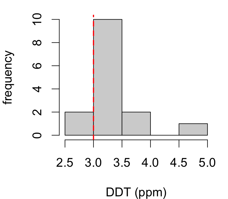
With only 15 observations, it’s hard to assess normality.

sign.test(ddt, m = 3, alternative = 'greater')
sample median: 3.22
hypothesis: m = 3
alternative: greater
p-value: 0.003692626953125

The data provide evidence that median DDT in kale exceeds 3ppm (p = 0.019).

Example: rank sum test

Is there a difference in serum cholesterol between corn flake and oat bran diets?
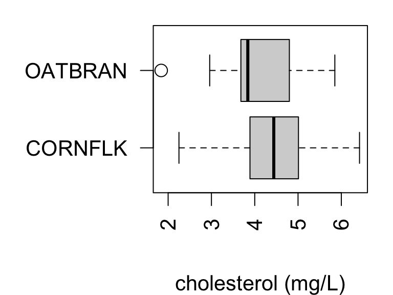
The oat bran group is right-skewed with outliers.

wilcox.test(cholesterol ~ diet, data = cholesterol)

    Wilcoxon rank sum exact test

data:  cholesterol by diet
W = 126, p-value = 0.2056
alternative hypothesis: true location shift is not equal to 0

The data provide no evidence of a difference in cholesterol between diets (rank sum test, p = 0.74).

Example: Kruskal-Wallis test

Does the distribution of AAM lengths differ by geographic location?
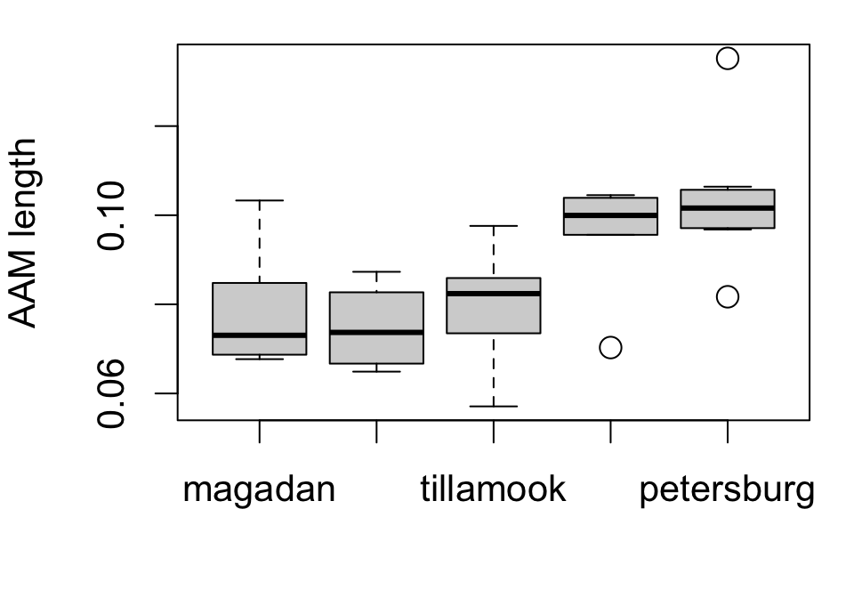
Small samples, unequal spreads, outliers, and skewness.

kruskal.test(aam.length ~ location, data = mussels)

    Kruskal-Wallis rank sum test

data:  aam.length by location
Kruskal-Wallis chi-squared = 16.405, df = 4, p-value = 0.002521

The data provide evidence that the distribution of AAM lengths differs by geographic location (Kruskal-Wallis test, p = 0.0025).

Linear regression

The method

Data: paired measurements of two continuous variables (one response, one explanatory).

Model: \(\quad y = \beta_0 + \beta_1 x + \epsilon\)

Parameters: intercept \(\beta_0\), slope \(\beta_1\)

Inference for the slope:

\[ \begin{cases} H_0: &\beta_1 = 0 \quad\text{(no association)} \\ H_A: &\beta_1 \neq 0 \end{cases} \qquad T = \frac{\hat\beta_1}{SE(\hat\beta_1)} \sim t_{n - 2} \]

Predictions:

  • confidence interval for the mean response at \(x^*\)
  • prediction interval for an individual response at \(x^*\)

Example: cognitive function and age

How much does RFFT score decline with age? (PREVEND data)
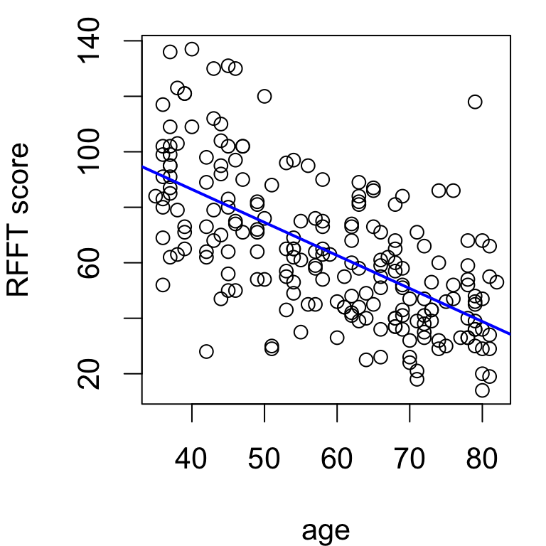
fit.prevend <- lm(rfft ~ age, data = prevend)
summary(fit.prevend)

Call:
lm(formula = rfft ~ age, data = prevend)

Residuals:
    Min      1Q  Median      3Q     Max 
-56.085 -14.690  -2.937  12.744  77.975 

Coefficients:
            Estimate Std. Error t value Pr(>|t|)    
(Intercept) 134.0981     6.0701   22.09   <2e-16 ***
age          -1.1908     0.1007  -11.82   <2e-16 ***
---
Signif. codes:  0 '***' 0.001 '**' 0.01 '*' 0.05 '.' 0.1 ' ' 1

Residual standard error: 20.52 on 206 degrees of freedom
Multiple R-squared:  0.4043,    Adjusted R-squared:  0.4014 
F-statistic: 139.8 on 1 and 206 DF,  p-value: < 2.2e-16

With each additional year of age, mean RFFT score decreases by an estimated 1.19 points.

Inference and prediction

confint(fit.prevend)
                 2.5 %      97.5 %
(Intercept) 122.130647 146.0654574
age          -1.389341  -0.9922471

With 95% confidence, each additional year of age is associated with a decrease in mean RFFT score of between 0.99 and 1.39 points.

predict(fit.prevend, newdata = data.frame(age = 55), interval = 'prediction')
       fit      lwr      upr
1 68.60439 28.04903 109.1598

With 95% confidence, the RFFT score for an individual 55 year old is estimated to be between 28 and 109.2 points.

Inference for categorical data

One-sample inference

Data: \(n\) observations of a categorical variable with \(k\) categories.

  • \(k = 2\): binomial data
  • \(k > 2\): multinomial data

Parameter: population proportions \(\mathbf{p} = (p_1, \dots, p_k)\)

Test statistic: \(\quad \chi^2 = \sum_i \dfrac{(O_i - E_i)^2}{E_i}\)

where \(O_i\) = observed count and \(E_i\) = expected count under \(H_0: \mathbf{p} = \mathbf{p}_0\).

Sampling distribution: \(\quad \chi^2_{k - 1}\) model

Confidence interval for \(p_k\): \(\quad \hat{p}_k \pm c \times \sqrt{\dfrac{\hat{p}_k(1 - \hat{p}_k)}{n}}\)

Example: diabetes prevalence

Is diabetes prevalence in the U.S. equal to 10%?
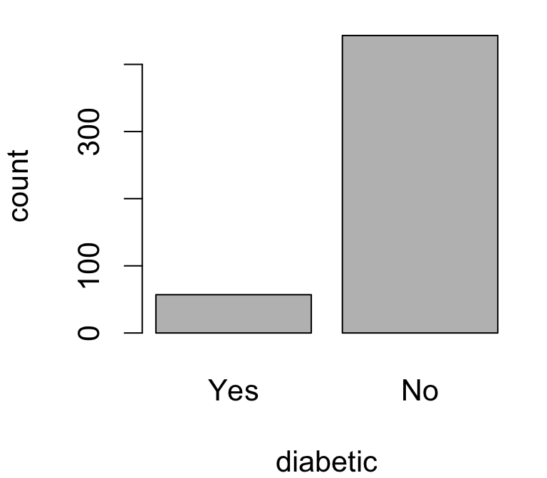
prop.test(x = 57, n = 500, p = 0.10)

    1-sample proportions test with continuity correction

data:  57 out of 500, null probability 0.1
X-squared = 0.93889, df = 1, p-value = 0.3326
alternative hypothesis: true p is not equal to 0.1
95 percent confidence interval:
 0.08814952 0.14594579
sample estimates:
    p 
0.114 

The data provide no evidence that diabetes prevalence differs from 10% (\(\chi^2\) = 0.94 on 1 degree of freedom, p = 0.33). With 95% confidence, diabetes prevalence among U.S. adults is estimated to be between 8.8% and 14.6%.

Multi-sample or grouped inference

Data: \(J\) groups of \(n_j\) observations of a categorical variable with \(k\) categories.

Parameter: group/sample proportions \(\mathbf{p}_1, \dots, \mathbf{p}_J\)

Test statistic: \(\quad \chi^2 = \sum_{i, j} \dfrac{(O_{ij} - E_{ij})^2}{E_{ij}}\)

where \(O\) = observed count, \(E\) = expected count under \(H_0: \mathbf{p}_1 = \cdots = \mathbf{p}_J\)

Residuals explain where an association/difference lies: \(\quad r_{ij} = \dfrac{O_{ij} - E_{ij}}{\sqrt{E_{ij}}}\)

Measures of association for \(2 \times 2\) tables:

  • Relative risk: \(\widehat{RR} = \frac{\hat{p}_1}{\hat{p}_2}\)
  • Odds ratio: \(\hat{\omega} = \frac{\hat{p}_1/(1 - \hat{p}_1)}{\hat{p}_2/(1 - \hat{p}_2)}\)

Example: genotype and race

Do ACTN3 genotype frequencies vary by race? (FAMuSS data)

  CC CT TT
African Am 16 6 5
Asian 21 18 16
Caucasian 125 216 126
Hispanic 4 10 9
Other 7 11 5
table(famuss$race, famuss$genotype) |>
  chisq.test()

    Pearson's Chi-squared test

data:  table(famuss$race, famuss$genotype)
X-squared = 19.4, df = 8, p-value = 0.01286

The data provide evidence of an association between race and genotype (\(\chi^2\) = 19.4 on 8 degrees of freedom, p = 0.013).

Residual analysis

Which combinations drive the association?

chisq.test(tbl)$residuals |> round(2)
            genotype
race            CC    CT    TT
  African Am  2.91 -1.70 -0.85
  Asian       1.25 -1.25  0.29
  Caucasian  -0.93  0.78 -0.03
  Hispanic   -1.04 -0.03  1.11
  Other       0.12  0.29 -0.49

African American and Asian populations have higher CC and lower CT frequencies than would be expected if genotype were independent of race.

Example: relative risk

Does asthma prevalence differ by sex?

table(asthma$sex, asthma$asthma) |>
  ratio.test(outcome = 'asthma', 
             group = 'female',
             measure = 'rr', 
             conf.level = 0.90)
Risk comparison
  Outcome : asthma
  Group   : female  (vs. male)
  Measure : Relative risk

        
         no asthma asthma
  male         769     30
  female       781     49

Relative risk = 1.5723  (90% CI: 1.0834, 2.2820)

Chi-squared test of association:
  X-squared = 4.0741, df = 1, p-value = 0.04355
  asthma no asthma
male 30 769
female 49 781

The data provide evidence of an association between asthma and sex (\(\chi^2\) = 3.62 on 1 degree of freedom, p = 0.057). With 90% confidence, the risk of asthma is estimated to be between 1.08 and 2.28 times greater for women than for men, with a point estimate of 1.57.

Example: odds ratio

Is smoking associated with lung cancer?

table(smoking$smoking, smoking$group) |>
  ratio.test(outcome = 'Cancer', 
             group = 'Smokers',
             measure = 'or')
Risk comparison
  Outcome : Cancer
  Group   : Smokers  (vs. NonSmokers)
  Measure : Odds ratio

            
             Control Cancer
  NonSmokers      14      3
  Smokers         72     83

Odds ratio = 5.3796  (95% CI: 1.4864, 19.4705)

Chi-squared test of association:
  X-squared = 7.8983, df = 1, p-value = 0.004948
  Smokers NonSmokers
Cancer 83 3
Control 72 14

The data provide evidence of an association between smoking and lung cancer (\(\chi^2 = 6.53\) on 1 degree of freedom, \(p = 0.0106\)). With 95% confidence, the relative odds of cancer are estimated to be between 1.49 and 19.47 times greater among smokers compared with nonsmokers, with a point estimate of 5.38.

Wrapping up

Common threads

Across every method:

  • Same logic: estimate → standardize → compare to reference distribution → p-value
  • Same interpretation style: evidence statement + interval estimate, always in context
  • Same assumptions to check: independence of observations, distributional shape, sample size
  • Same limitation: tests tell you whether an effect exists, not how big it is — always pair with confidence intervals or effect sizes

Extensions: multiple regression

What if we have more than one explanatory variable?

\[\text{% change} = \beta_0 + \beta_1\, \text{age} + \beta_2\; \text{sex} + \epsilon\]
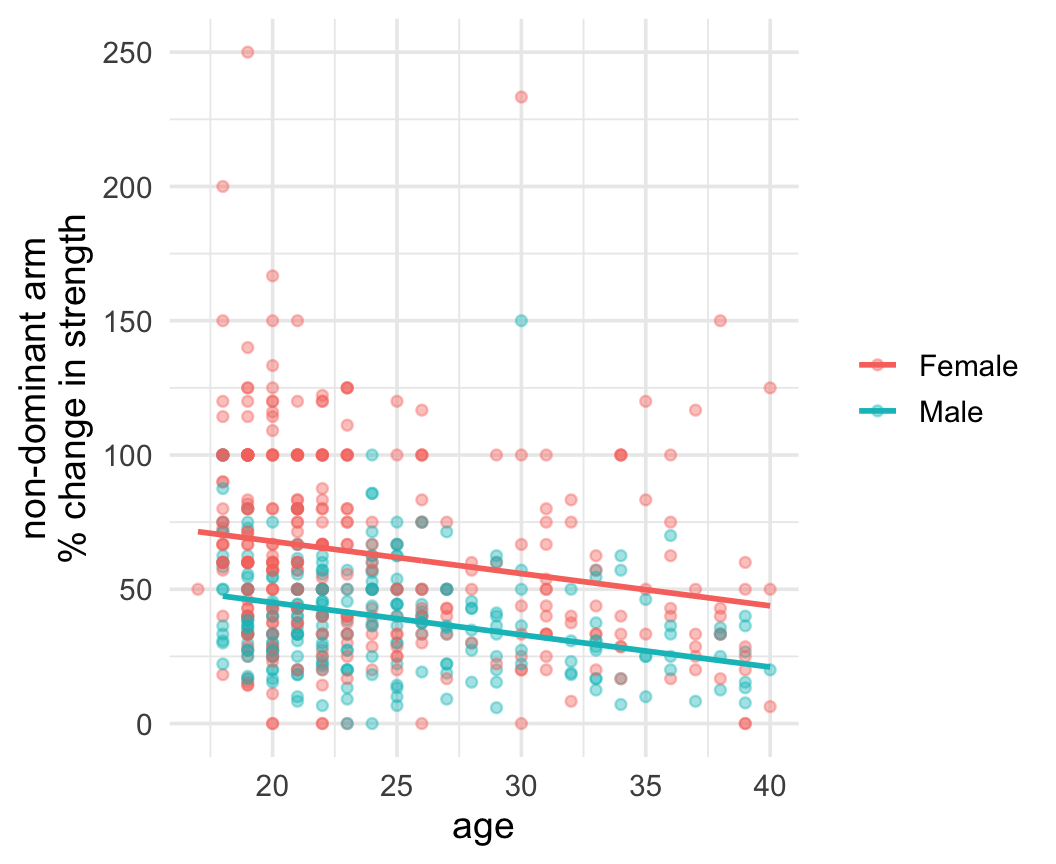
fit <- lm(ndrm.ch ~ age + sex, data = famuss)
coef(fit) |> round(2)
(Intercept)         age     sexMale 
      91.86       -1.20      -22.80 

Each line represents the relationship between age and strength gain after adjusting for sex.

  • Females gain ~22% more strength than males of the same age
  • Each additional year of age is associated with ~1% less strength gain

Extensions: two-way ANOVA

What if we have two grouping variables — and they might interact?
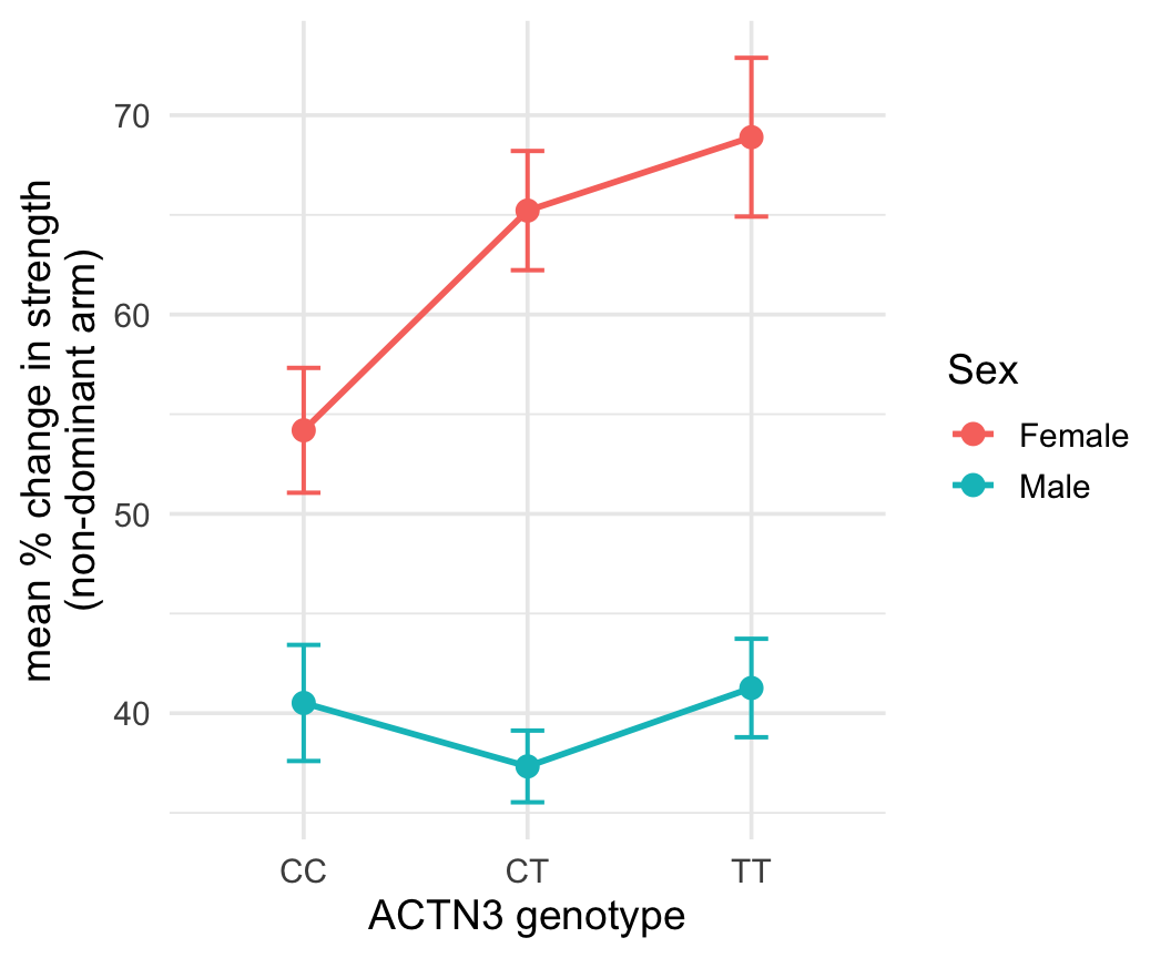
fit <- aov(ndrm.ch ~ genotype * sex, data = famuss)
summary(fit)
              Df Sum Sq Mean Sq F value Pr(>F)    
genotype       2   7043    3522   3.713 0.0250 *  
sex            1  80847   80847  85.246 <2e-16 ***
genotype:sex   2   5837    2918   3.077 0.0468 *  
Residuals    589 558609     948                   
---
Signif. codes:  0 '***' 0.001 '**' 0.01 '*' 0.05 '.' 0.1 ' ' 1
  • Interaction: does the genotype effect differ by sex?
  • Parallel lines → no interaction
  • Non-parallel lines → interaction present

Future courses

If you want to learn more, consider a minor. Core coursework after STAT218:

  • Statistical computing with R (STAT1810)
  • Statistics II (STAT3520)
  • 3 electives
    • data science (DATA3301), regression (STAT3430), experimental design (STAT3540)
    • (just my suggestions)

For more info: https://statistics.calpoly.edu/content/minors