# A tibble: 6 × 5
  genhlth   gender   age wtdesire weight
  <fct>     <fct>  <int>    <int>  <int>
1 very good m         45      225    265
2 excellent m         24      150    150
3 excellent m         47      150    137
4 good      f         26      125    159
5 very good f         33      125    145
6 very good f         28      120    125
1. Observational data. Researchers measured existing health characteristics from a sample of U.S. adults; no treatment was assigned.
Part 1: General health
table(brfss$genhlth)
   excellent    very good         good fair or poor
          17           18           17            8
2. Ordinal: it is categorical because its values are qualitative, and the values are ordered because, e.g., good exceeds fair/poor.
     excellent  very good       good fair or poor
  m  1.6687175 -0.2373222 -0.7733081   -0.9492889
  f -1.6139905  0.2295390  0.7479468    0.9181562
4. The data provide evidence of an association between self-reported general health and gender (\(\chi^2\) = 8.4 on 3 degrees of freedom, p = 0.0384). The residuals indicate that more men and fewer women than expected under independence report themselves as being in excellent health.
table(brfss$gender, brfss$genhlth)
    excellent very good good fair or poor
  m        13         8    6            2
  f         4        10   11            6
5.\(\frac{13}{29}\) men and \(\frac{4}{31}\) women, or 44.8% and 12.9%, respectively, report being in excellent health.
6. Rewrite the table as a 2×2: excellent vs. other rating.
excellent
other.rating
m
13
16
f
4
27
The odds for men are \(\frac{13}{16}\), the odds for women are \(\frac{4}{27}\), so the odds ratio is \(\hat{\omega} = \frac{13/16}{4/27} = 5.48\).
For the interval:
The standard error for the log odds ratio is \(SE(\log(\hat{\omega})) = \sqrt{\frac{1}{13} + \frac{1}{16} + \frac{1}{4} + \frac{1}{27}} = 0.653\).
The confidence interval for the log odds ratio is \(\log(5.48) \pm 2\times 0.653 = (0.395, 3.007)\).
Exponentiating endpoints yields an interval for the odds ratio of \((1.48, 20.23)\).
With 95% confidence, men are between 1.48 and 20.23 times more likely than women to report being in excellent health.
Part 2: Weight loss motivation
fit <-aov(weight - wtdesire ~ genhlth, data = brfss)summary(fit)
            Df Sum Sq Mean Sq F value Pr(>F)
genhlth      3   7395    2465   2.353 0.0818 .
Residuals   56  58657    1047
---
Signif. codes:  0 '***' 0.001 '**' 0.01 '*' 0.05 '.' 0.1 ' ' 1
7. No, the data do not provide evidence that mean desired weight loss differs by self-reported general health (F = 2.35 on 3 and 56 df, p = 0.0818).
 genhlth      emmean    SE df lower.CL upper.CL
 excellent      5.53  7.85 56   -14.73     25.8
 very good     16.56  7.63 56    -3.13     36.2
 good          34.47  7.85 56    14.21     54.7
 fair or poor  14.38 11.40 56   -15.16     43.9

Confidence level used: 0.95
Conf-level adjustment: bonferroni method for 4 estimates
8. The mean desired weight loss among U.S. adults who rate themselves as being in excellent general health is estimated to be 5.53 lbs; with 95% confidence, this figure is estimated to be between a weight gain of 14.73 lbs and a weight loss of 25.8 lbs.
9. Good only. The conclusion of a 5% level two-sided test of \(H_0: \mu_i = 0\) can be inferred from whether the 95% intervals span zero. Only the good category has an interval estimate for mean desired weight loss that is strictly positive.
kruskal.test(weight - wtdesire ~ genhlth, data = brfss)
    Kruskal-Wallis rank sum test

data:  weight - wtdesire by genhlth
Kruskal-Wallis chi-squared = 6.0081, df = 3, p-value = 0.1112
10. The “good” group exhibits more variability than the others with respect to desired weight loss and includes two very large outliers. While the conclusions do not differ at the 5% level, they would at the 10% level.
Part 3: Weight loss and gender
mean(brfss$weight - brfss$wtdesire)
[1] 18.21667
sd(brfss$weight - brfss$wtdesire)
[1] 33.45936
11. The interval is \(18.22 \pm 2\times\frac{33.46}{\sqrt{60}} = (9.58, 26.86)\).
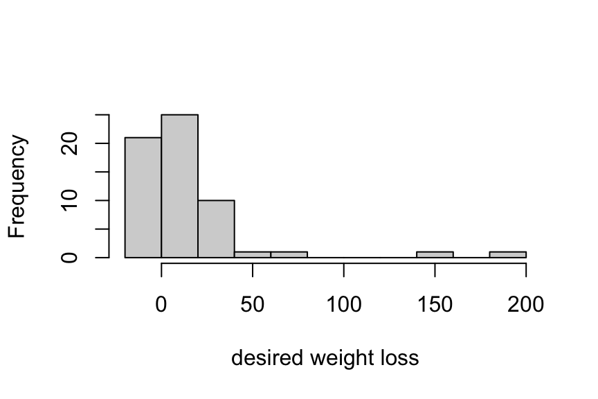
12. Right-skewed and unimodal, with a few large outliers.
13. It’s questionable. The sample size is large enough that the \(t\)-test may work fine, but the outliers are concerning and may affect results.
t.test(brfss$weight - brfss$wtdesire,mu =0, alternative ='greater')
    One Sample t-test

data:  brfss$weight - brfss$wtdesire
t = 4.2172, df = 59, p-value = 4.311e-05
alternative hypothesis: true mean is greater than 0
95 percent confidence interval:
 10.99824      Inf
sample estimates:
mean of x
 18.21667
wilcox.test(brfss$weight - brfss$wtdesire,mu =0, alternative ='greater')
    Wilcoxon signed rank test with continuity correction

data:  brfss$weight - brfss$wtdesire
V = 867.5, p-value = 9.799e-08
alternative hypothesis: true location is greater than 0
14. We want the greater alternative since a positive value for \(\mu\) means that actual weight exceeds desired weight. The nonparametric test is the better choice here (see previous solution) but either is acceptable.
The data provide evidence that the typical U.S. adult wishes to lose weight (signed rank test, p < 0.0001).
t.test(weight - wtdesire ~ gender, data = brfss)
    Welch Two Sample t-test

data:  weight - wtdesire by gender
t = -2.048, df = 38.875, p-value = 0.04735
alternative hypothesis: true difference in means between group m and group f is not equal to 0
95 percent confidence interval:
 -33.4685580  -0.2066366
sample estimates:
mean in group m mean in group f
       9.517241       26.354839
wilcox.test(weight - wtdesire ~ gender, data = brfss)
    Wilcoxon rank sum exact test

data:  weight - wtdesire by gender
W = 288.5, p-value = 0.01495
alternative hypothesis: true location shift is not equal to 0
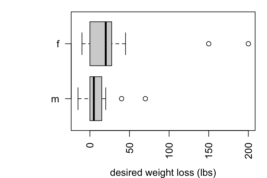
15. The nonparametric test is more appropriate owing to the outliers. The data provide evidence that typical desired weight loss differs by gender (rank sum test, p = 0.0159).
Part 4: Age and weight
cor(brfss$age, brfss$weight)
[1] 0.09502067
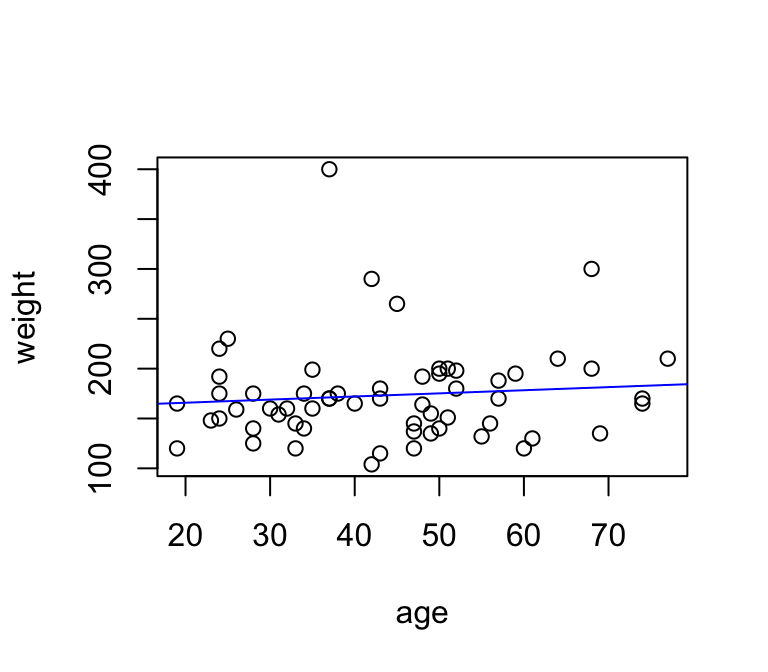
16. There is essentially no linear relationship between weight and age (\(r = 0.095\)).
fit <-lm(weight ~ age, data = brfss)summary(fit)
Call:
lm(formula = weight ~ age, data = brfss)

Residuals:
    Min      1Q  Median      3Q     Max
-68.744 -29.545  -8.087  17.796 228.828

Coefficients:
            Estimate Std. Error t value Pr(>|t|)
(Intercept) 159.5339    19.9751   7.987 6.45e-11 ***
age           0.3145     0.4327   0.727     0.47
---
Signif. codes:  0 '***' 0.001 '**' 0.01 '*' 0.05 '.' 0.1 ' ' 1

Residual standard error: 49.23 on 58 degrees of freedom
Multiple R-squared:  0.009029,  Adjusted R-squared:  -0.008057
F-statistic: 0.5284 on 1 and 58 DF,  p-value: 0.4702
17. The data provide no evidence of a relationship between mean weight and age (T = 0.727 on 58 df, p = 0.47).
18. Age explains an estimated 0.9% of variation in weight.
19. The estimate and standard error are shown in the output:
$data
           Outcome
Predictor   no CHD CHD Total
  nonsmoker   4913  87  5000
  smoker      2916  84  3000
  Total       7829 171  8000

$measure
           risk ratio with 95% C.I.
Predictor   estimate    lower    upper
  nonsmoker 1.000000       NA       NA
  smoker    1.609195 1.196452 2.164325
23. Smokers are an estimated 1.61 times as likely to develop CHD compared with nonsmokers (RR = 1.61, 95% CI: 1.20 to 2.16). With 95% confidence, the risk of CHD among smokers is between 1.20 and 2.16 times that of nonsmokers; because the interval excludes 1, the data provide evidence of an association between smoking and CHD risk.
24. Efficacy is \(1 - \frac{1}{RR} = 1 - \frac{1}{1.61} = 0.379\), or about 38%. Not smoking reduces the risk of CHD by an estimated 38% compared with smoking.
Part 6: Mammalian metabolic rates
metab <- ex0826
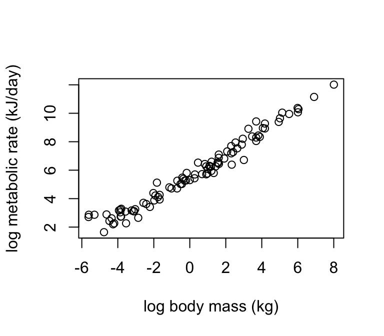
25. There is a strong, positive, linear trend: mammal species with larger log body mass tend to have larger log metabolic rates.
fit.metab <-lm(log(Metab) ~log(Mass), data = metab)summary(fit.metab)
Call:
lm(formula = log(Metab) ~ log(Mass), data = metab)

Residuals:
     Min       1Q   Median       3Q      Max
-1.14216 -0.26466 -0.04889  0.25308  1.37616

Coefficients:
            Estimate Std. Error t value Pr(>|t|)
(Intercept)  5.63833    0.04709  119.73   <2e-16 ***
log(Mass)    0.73874    0.01462   50.53   <2e-16 ***
---
Signif. codes:  0 '***' 0.001 '**' 0.01 '*' 0.05 '.' 0.1 ' ' 1

Residual standard error: 0.4572 on 93 degrees of freedom
Multiple R-squared:  0.9649,    Adjusted R-squared:  0.9645
F-statistic:  2553 on 1 and 93 DF,  p-value: < 2.2e-16