# load datasets
load('data/famuss.RData')
load('data/nhanes.RData')
load('data/temps2.RData')Lab 2: Descriptive statistics and estimation
With solutions
ImportantBefore you begin
Fill in the author and calpoly-id fields at the very top of this file. Replace "Your Name Here" with your full name and "yourpolynetid" with your Cal Poly username (the part of your email before @calpoly.edu, e.g. jdoe01). Your submission cannot be matched to your record without this.
Where a “Your turn” asks you to save a result by a specific name (shown in bold), use the exact name given — your work is checked automatically.
Descriptive statistics
The FAMuSS study recruited young adults to examine how genetic variation affects muscle strength gains from resistance training. We’ll use this dataset throughout.
Histograms
How old were participants when they enrolled in FAMuSS?
For numeric variables, hist() bins observations into intervals to show the shape of the distribution. The breaks argument controls the number of bins.
# extract age variable
age <- famuss$age

# default histogram
hist(age)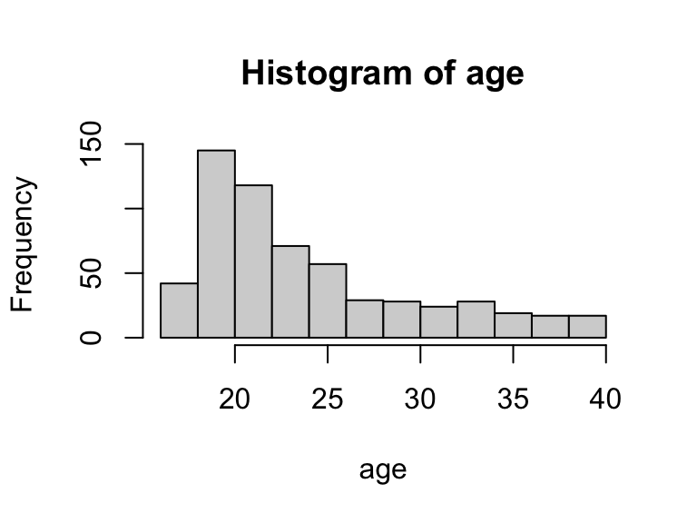
# more bins — finer detail
hist(age, breaks = 20)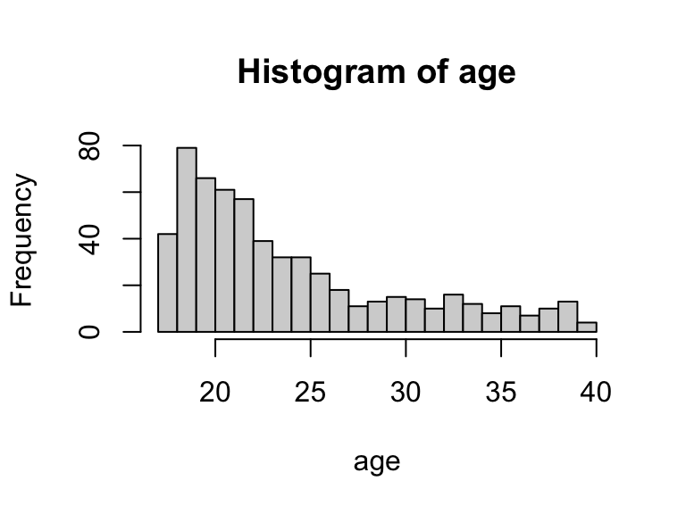
# fewer bins — broader shape
hist(age, breaks = 5)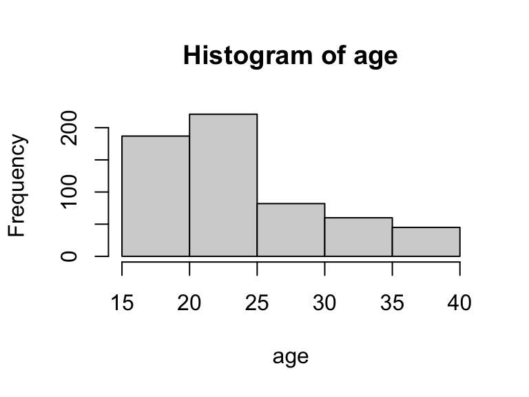
CautionYour turn 1 [L3]
How much did participants’ nondominant arm strength change over the course of the training program — was there consistent improvement?
Extract ndrm.ch (percent change in nondominant arm strength) from famuss and construct a histogram. Tinker with the breaks argument to find a setting that captures the shape well. Is the distribution skewed or symmetric?
TipSolution
# extract ndrm.ch variable
ndrm.ch <- famuss$ndrm.ch

# construct histogram
hist(ndrm.ch, breaks = 20)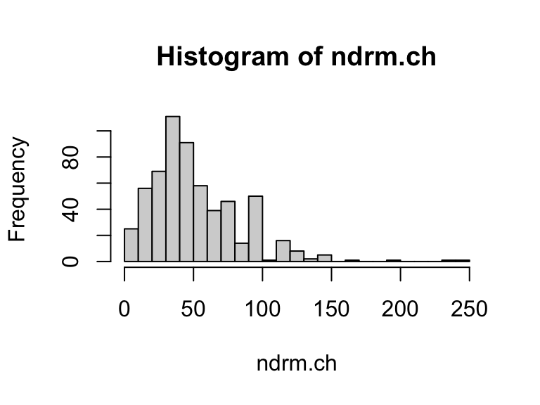
The distribution is right-skewed. Around 20 breaks captures the shape well.
Summary statistics
Beyond shape, we often want a few numbers to summarize where the distribution is centered and how spread out it is. summary() returns the five-number summary plus the mean in one call.
# five-number summary + mean for age
summary(age)
Min. 1st Qu. Median Mean 3rd Qu. Max.
17.0 20.0 22.0 24.4 27.0 40.0
CautionYour turn 2 [L3]
Compute summary statistics for ndrm.ch using summary(). Store the result as ndrm.summary.
What is the best way to characterize the typical percent change in strength? (Hint: look at your histogram from Your turn 1.)
TipSolution
# five-number summary + mean for ndrm.ch
ndrm.summary <- summary(ndrm.ch)
ndrm.summary
Min. 1st Qu. Median Mean 3rd Qu. Max.
0.00 30.00 45.50 53.29 66.70 250.00 The distribution is right-skewed, so the median is the better measure of center. The median percent change in nondominant arm strength was about 15%.
Estimating a population mean
The goal here shifts from describing a sample to making inferences about a broader population. The NHANES survey is designed to be representative of the U.S. adult population.
What is the mean total cholesterol level among U.S. adults?
t.test() computes a point estimate and standard error for a population mean in one step.
# extract total cholesterol
totchol <- nhanes$totchol

# run one-sample t-test — stores the full result
totchol.tt <- t.test(totchol)

# point estimate (sample mean)
totchol.tt$estimate
mean of x
5.042938 # standard error
totchol.tt$stderr[1] 0.01906042Interpreted as a point estimate of the population mean:
Mean total cholesterol of U.S. adults is estimated to be 5.04 mmol/L (SE 0.019).
CautionYour turn 3 [L4]
It’s long been claimed that normal human body temperature is 98.6°F — but is that accurate?
The temps dataset comes from a study that set out to answer exactly this question. Use t.test() on body temperature (body.temp) and store the result as bodytemp.tt. Print the point estimate and standard error. Write a one-sentence interpretation of the point estimate.
TipSolution
# extract body temperature
bodytemp <- temps$body.temp

# run t-test
bodytemp.tt <- t.test(bodytemp)

# point estimate and standard error
bodytemp.tt$estimate
mean of x
98.24923 bodytemp.tt$stderr[1] 0.06430442Mean body temperature is estimated to be 98.25°F (SE 0.064).
NoteSubmitting this assignment
- Save the file (Ctrl+S / Cmd+S).
- Render to PDF: click Render or press Ctrl+Shift+K / Cmd+Shift+K.
- Download both files: in the Files panel, check the
.qmdand PDF, then click More ▾ → Export…. - Upload the PDF to the Gradescope assignment.
- Upload the
.qmdfile to the course submission link.