Lab 3: Point and interval estimation

Course activity

STAT218

library(tidyverse)
load('data/nhanes.RData')
load('data/temps2.RData')

The goal of this lab is to learn to compute a point estimate, standard error, and interval estimate for a population mean “by hand” by performing the arithmetic directly in R. You will have an opportunity to practice interpreting these quantities as you go.

We will also use this lab for a short class activity to explore how often the interval estimate we introduced is “correct”.

Point estimation

Estimate for the population mean

Since the point estimate for the population mean of a numeric variable is the sample mean, you already know how to perform the calculation in R. We’ll store this for later use:

# retrieve total cholesterol variable
totchol <- nhanes$totchol

# store sample mean as totchol.mean
totchol.mean <- mean(totchol)

# print
totchol.mean

[1] 5.042938

The only novelty here is that we now interpret this as a point estimate of the population mean total cholesterol:

The mean total cholesterol of U.S. adults is estimated to be 5.043 mmol/L.

This is in contrast to the interpretation as a descriptive summary:

The average total cholesterol among the respondents in the NHANES survey was 5.043 mmol/L.

Both interpretations are valid, just different. By interpreting the sample mean as a point estimate, we are implicitly assuming that the data are a random sample from the U.S. adult population.

Your turn

Use the temps data to compute average body temperature. Store the result as bodytemp.mean. How would you interpret the result differently…

as a descriptive summary?
as a point estimate?

Solution

# retrieve variable of interest
bodytemp <- temps$body.temp

# store sample mean as bodytemp.mean
bodytemp.mean <- mean(bodytemp)

# print
bodytemp.mean

[1] 98.24923

As a descriptive summary, we’d say that the average body temperature of study participants was 98.25 degrees Farenheit.

As a point estimate, we’d say that mean body temperature is estimated to be 98.25 degrees Farenheit.

Standard error for the sample mean

A standard error is a measure of the sampling variability of a point estimate. Technically, it’s an estimate of the point estimate’s standard deviation across all possible random samples of a fixed size.

The standard error for the sample mean is calculated according to the formula: \[SE(\bar{x}) = \frac{s_x}{\sqrt{n}}\] Where:

\(s_x\) is the sample standard deviation
\(n\) is the sample size

To calculate this in R, we perform the arithmetic by hand (for now):

# store sample sd and sample size
totchol.sd <- sd(totchol)
totchol.n <- length(totchol)

# compute standard error
totchol.se <- totchol.sd/sqrt(totchol.n)

# print
totchol.se

[1] 0.01906042

Recall that this is an estimate of the variability of the sample mean. The convention in scientific writing is to report the standard error parenthetically with the point estimate.

The mean total cholesterol of U.S. adults is estimated to be 5.043 mmol/L (SE 0.0191).

Qualitatively, that means that the point estimate for mean cholesterol varies around the target parameter by 0.0191 mmol/L on average.

Your turn

Calculate and the standard error for the sample mean of the body temperature variable.

Report the point estimate and standard error following conventional style.

Solution

# store sample sd and sample size
bodytemp.sd <- sd(bodytemp)
bodytemp.n <- length(bodytemp)

# compute standard error
bodytemp.se <- bodytemp.sd/sqrt(bodytemp.n)

# print
bodytemp.se

[1] 0.06430442

Mean body temperature is estimated to be 98.25 degrees Farenheit (SE 0.064).

Interval estimation

Interval estimate for the mean

A common interval for the population mean is:

\[\bar{x} \pm \underbrace{2\times SE(\bar{x})}_{\text{margin of error}}\]

For now, we’ll calculate this by directly performing the arithmetic. Later, you’ll use commands that return interval estimates by default.

# interval estimate for mean total cholesterol
totchol.mean - 2*totchol.se

[1] 5.004817

totchol.mean + 2*totchol.se

[1] 5.081059

We interpret this result as follows:

Mean total cholesterol of U.S. adults is estimated to be between 5.005 and 5.081 mmol/L.

A handy shortcut in R is to use vectorized arithmetic to compute both the lower and upper bound in one line:

# interval estimate for mean total cholesterol
totchol.mean + c(-2, 2)*totchol.se

[1] 5.004817 5.081059

Your turn

Calculate an interval estimate for the mean body temperature using the body temperature data and interpret the interval in context.

Solution

# interval estimate for mean body temp
bodytemp.mean + c(-2, 2)*bodytemp.se

[1] 98.12062 98.37784

Mean body temperature is estimated to be between 98.12 and 98.38 degrees Farenheit.

Extra: exploring sex differences

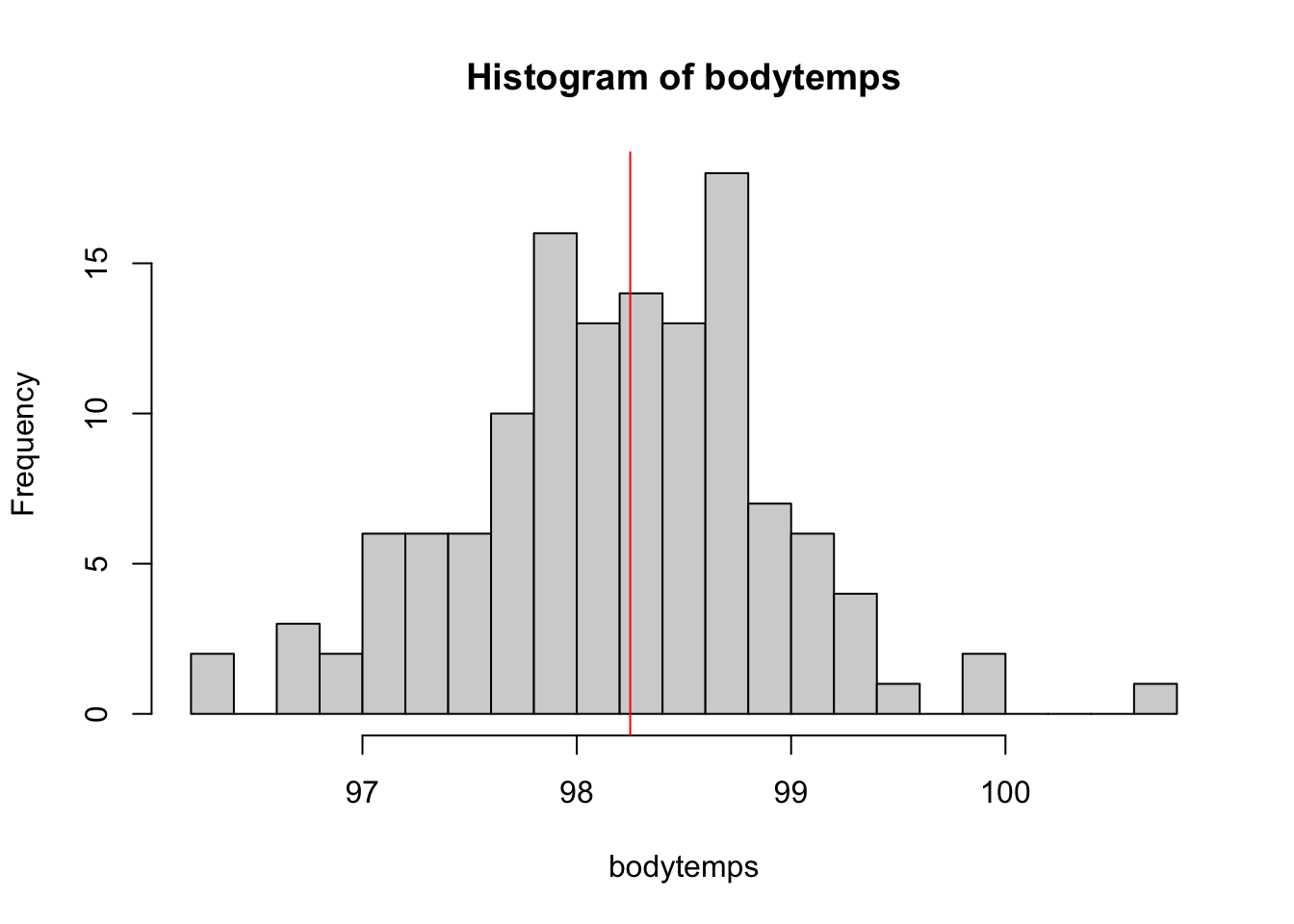
Have a look at the distribution of body temperatures:

# body temperatures
bodytemps <- temps$body.temp

# histogram of body temps with sample mean overlaid
hist(bodytemps, breaks = 30)
abline(v = mean(bodytemps), col = 'red')

Notice that there are two distinct peaks – the distribution appears to be bimodal. One possible explanation is that the distribution of body temperatures differs by sex. Let’s explore that possibility.

The following cell partitions the data by sex:

# partition by sex
bodytemps.split <- split(temps$body.temp, temps$sex)
bodytemps.f <- bodytemps.split$female
bodytemps.m <- bodytemps.split$male

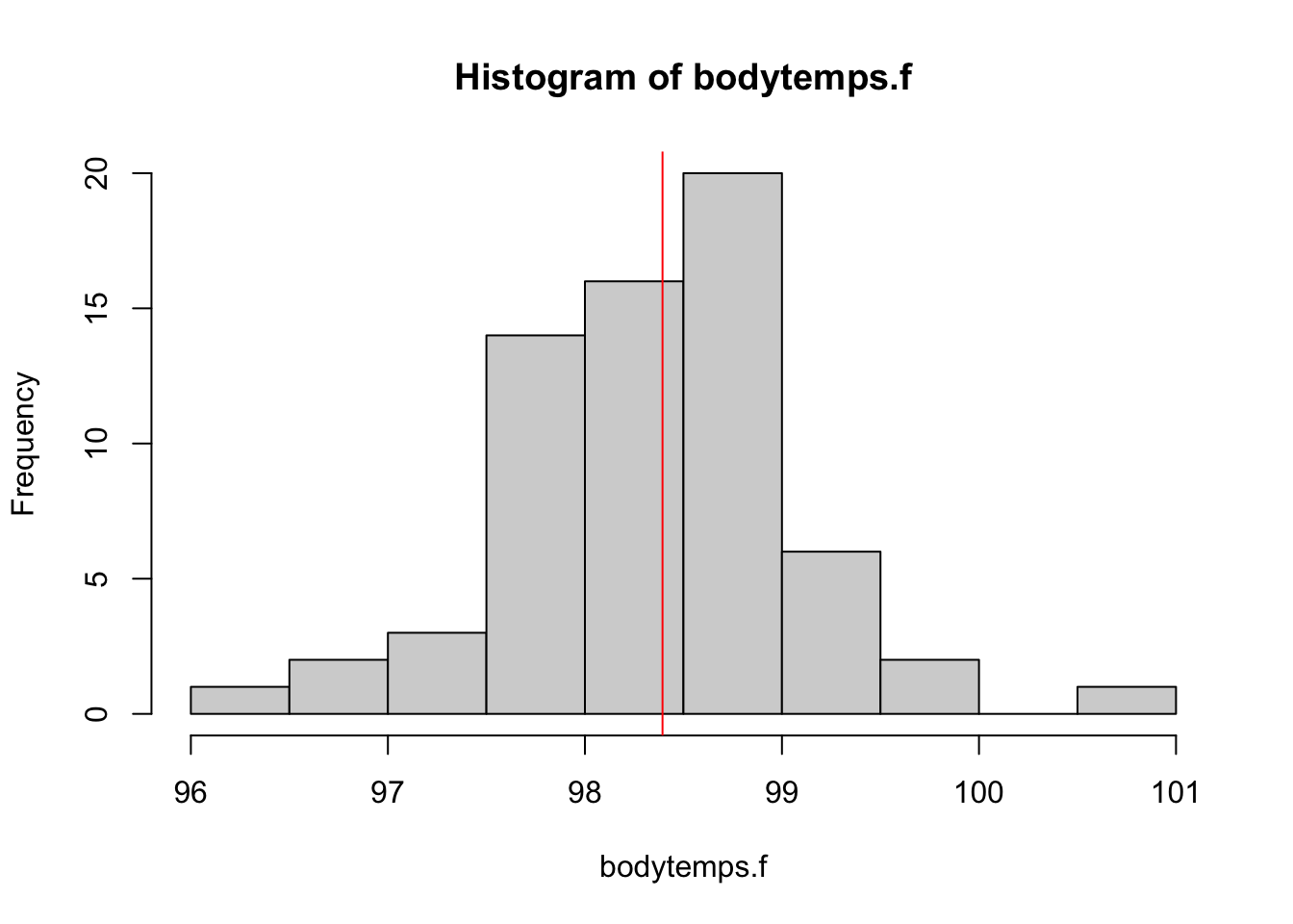
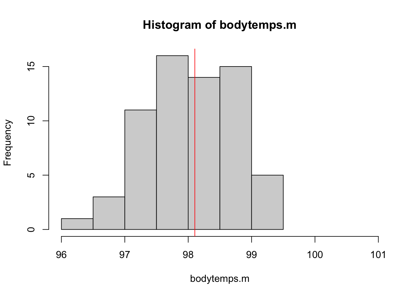
Now let’s compare the distributions of body temperatures:

# distribution of female body temperatures
hist(bodytemps.f, breaks = 10)
abline(v = mean(bodytemps.f), col = 'red')

# distribution of male body temperatures
hist(bodytemps.m, breaks = 10, xlim = c(96, 101))
abline(v = mean(bodytemps.m), col = 'red')

The distribution of female body temperatures is generally shifted a bit to the right of the distribution of male body temperatures; likewise, the average is correspondingly slightly higher among females.

Your turn

Compute interval estimates for:

the mean body temperature of females
the mean body temperature of males

Comparing the interval estimates, do you think that a sex difference is present? Why or why not?

Solution

# interval for females
mean(bodytemps.f) + c(-2, 2)*sd(bodytemps.f)/length(bodytemps.f)

[1] 98.37097 98.41672

# interval for males
mean(bodytemps.m) + c(-2, 2)*sd(bodytemps.m)/length(bodytemps.m)

[1] 98.08312 98.12612

Since the intervals do overlap, it is reasonable to argue that there is not a sex difference: it is plausible that the means are the same.