load('data/census.RData')
load('data/temps.RData')
load('data/mussels.RData')
sign.test <- function(x, m, alternative = 'two.sided'){
  sgn <- sum(x <= m)
  n <- length(x)
  if(alternative == 'two.sided'){
    pval <- binom.test(x = sgn, n = n, p = 0.5, alternative = 'two.sided')$p.value
  }
  if(alternative == 'greater'){
    pval <- binom.test(x = sgn, n = n, p = 0.5, alternative = 'less')$p.value
  }
  if(alternative == 'less'){
    pval <- binom.test(x = sgn, n = n, p = 0.5, alternative = 'greater')$p.value
  }
  paste("sample median: ", median(x), '\n',
        "hypothesis: m = ", m, '\n',
        "alternative: ", alternative, '\n',
        "p-value: ", pval,
        sep = '') |>
    writeLines()
}Lab 8: Nonparametric inference
With solutions
ImportantBefore you begin
Fill in the author and calpoly-id fields at the very top of this file. Replace "Your Name Here" with your full name and "yourpolynetid" with your Cal Poly username (the part of your email before @calpoly.edu, e.g. jdoe01). Your submission cannot be matched to your record without this.
Where a “Your turn” asks you to save a result by a specific name (shown in bold), use the exact name given — your work is checked automatically.
One-sample inference
Sign test
Is the median different from a hypothesized value?
The sign test makes no assumptions about the shape of the distribution — use it when the data are skewed or otherwise non-normal and you want to test the median. The alternative argument accepts 'two.sided', 'greater', or 'less'.
Here’s an example testing whether median DDT in kale samples is 3:
# ddt data
ddt <- MASS::DDT

# sign test
sign.test(ddt, m = 3, alternative = 'two.sided')
sample median: 3.22
hypothesis: m = 3
alternative: two.sided
p-value: 0.00738525390625The data provide evidence that the median DDT in kale is not 3 ppm (sign test, p = 0.0074).
Is median personal income under $25K?
Income is strongly right-skewed, so the mean is unreliable — the sign test lets us test the median without any distributional assumption.
# personal incomes
income <- census$total_personal_income

# inspect distribution
hist(income)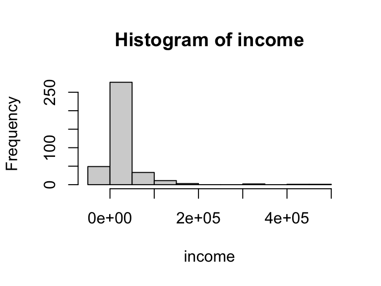
CautionYour turn 1
Using the census data, test whether median total personal income is less than 25K using the sign test. Interpret the result in context.
TipSolution
# sign test
sign.test(income, m = 25000, alternative = 'less')
sample median: 19604
hypothesis: m = 25000
alternative: less
p-value: 2.65434634358506e-06The data provide evidence that median income is under 25K.
Signed rank test
Is the center of a symmetric distribution different from a hypothesized value?
The signed rank test is more powerful than the sign test, but requires that the distribution be roughly symmetric. The syntax mirrors t.test() — use wilcox.test() instead.
Body temperatures are roughly symmetric, satisfying the signed rank test’s key assumption.
# body temperatures
btemp <- temps$body.temp

# check symmetry
hist(btemp)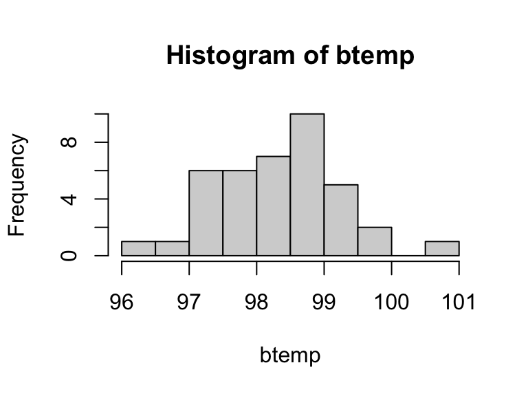
Here’s an example testing whether median body temperature is 98.7°F:
# signed rank test
btemp.srt <- wilcox.test(btemp, mu = 98.7, alternative = 'two.sided')

# show results
btemp.srt
    Wilcoxon signed rank exact test

data:  btemp
V = 243.5, p-value = 0.04086
alternative hypothesis: true location is not equal to 98.7
The data provide evidence that median body temperature is not 98.7 degrees Fahrenheit (signed rank test, p = 0.041).
Is median heart rate greater than 73 bpm?
Heart rates are also roughly symmetric.
# heart rates
hrate <- temps$heart.rate

# check symmetry
hist(hrate)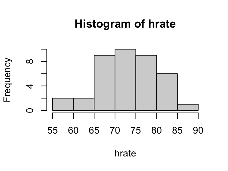
CautionYour turn 2 [L8]
Test whether median heart rate is greater than 73 bpm and interpret the result in context. Store the result as hrate.srt.
TipSolution
# signed rank test
hrate.srt <- wilcox.test(hrate, mu = 73, alternative = 'greater')

# show results
hrate.srt
    Wilcoxon signed rank exact test

data:  hrate
V = 459, p-value = 0.1651
alternative hypothesis: true location is greater than 73
The data do not provide evidence that median heart rate is greater than 73 bpm (signed rank test, p = 0.165).
Two-sample inference
Do the centers of two groups differ?
The rank sum test is a nonparametric alternative to the two-sample \(t\) test. Use it when the data contain heavy tails, substantial outliers, or clear skew. Like t.test(), it accepts a formula interface and one-sided alternatives.
Here’s an example testing whether body temperatures differ between men and women:
# rank sum test
wilcox.test(body.temp ~ sex, data = temps)
    Wilcoxon rank sum exact test

data:  body.temp by sex
W = 249.5, p-value = 0.09572
alternative hypothesis: true location shift is not equal to 0
The data do not provide evidence that body temperatures differ by sex (rank sum test, p = 0.097).
Are incomes higher among men than women?
Income distributions are heavily right-skewed with large outliers, making the rank sum test a better choice than the two-sample \(t\) test.
# income by sex
boxplot(total_personal_income ~ sex, data = census, horizontal = TRUE)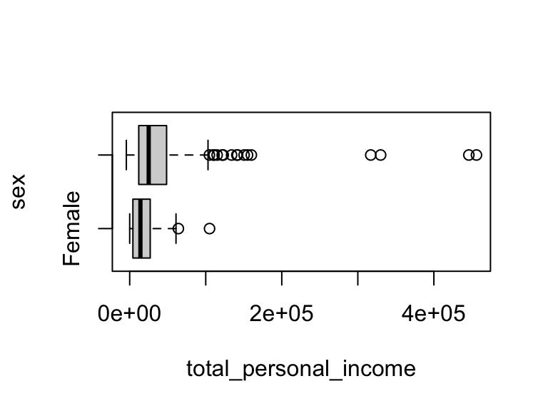
CautionYour turn 3 [L8]
Using the census data, test whether incomes are higher among men than among women. Store the result as income.rst. Interpret your result in context.
TipSolution
# rank sum test
income.rst <- wilcox.test(total_personal_income ~ sex, data = census, alternative = 'less')
income.rst
    Wilcoxon rank sum test with continuity correction

data:  total_personal_income by sex
W = 11889, p-value = 1.363e-08
alternative hypothesis: true location shift is less than 0
The data provide evidence that incomes are higher among men than women (rank sum test, p < 0.0001).
By including conf.int and conf.level arguments, we can obtain an estimate and confidence interval for the magnitude of the location shift:
# rank sum test with confidence interval
wilcox.test(body.temp ~ sex, data = temps, conf.int = TRUE, conf.level = 0.95)
    Wilcoxon rank sum exact test

data:  body.temp by sex
W = 249.5, p-value = 0.09572
alternative hypothesis: true location shift is not equal to 0
96.3 percent confidence interval:
 -0.2  1.1
sample estimates:
difference in location
                   0.5
Body temperatures are estimated to be about 0.5°F higher among women, but the 95% CI includes zero.
Kruskal-Wallis test
Do more than two groups differ in location?
The Kruskal-Wallis test is a nonparametric alternative to one-way ANOVA. Use it when the groups contain outliers or strong skew that would distort the \(F\) test. The mussel AAM length data, for example, shows outliers in several groups:
# aam lengths by location
boxplot(aam.length ~ location, data = mussels)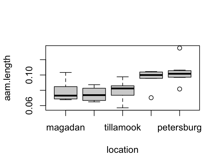
# kruskal-wallis test
kruskal.test(aam.length ~ location, data = mussels)
    Kruskal-Wallis rank sum test

data:  aam.length by location
Kruskal-Wallis chi-squared = 16.405, df = 4, p-value = 0.002521
Does personal income differ by race?
The same skew and outlier pattern holds across racial groups, motivating the Kruskal-Wallis test over ANOVA.
# income by race
boxplot(total_personal_income ~ race_general, data = census, horizontal = TRUE, las = 2, ylab = NULL)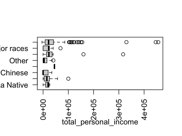
CautionYour turn 4 [L8]
Using the census data, test whether personal incomes differ by race. Store the result as income.kwt. Interpret your result in context.
TipSolution
# kruskal-wallis test
income.kwt <- kruskal.test(total_personal_income ~ race_general, data = census)
income.kwt
    Kruskal-Wallis rank sum test

data:  total_personal_income by race_general
Kruskal-Wallis chi-squared = 24.063, df = 7, p-value = 0.001111
The data provide evidence that personal income differs by race (Kruskal-Wallis test, p = 0.0011). Note that the parametric ANOVA does not reach the same conclusion — a consequence of the heavy-tailed income distributions distorting the \(F\) test.
# compare with parametric alternative
aov(total_personal_income ~ race_general, data = census) |> summary()
Df Sum Sq Mean Sq F value Pr(>F)
race_general 7 2.960e+10 4.228e+09 1.967 0.0586 .
Residuals 369 7.933e+11 2.150e+09
---
Signif. codes: 0 '***' 0.001 '**' 0.01 '*' 0.05 '.' 0.1 ' ' 1
NoteSubmitting this assignment
- Save the file (Ctrl+S / Cmd+S).
- Render to PDF: click Render or press Ctrl+Shift+K / Cmd+Shift+K.
- Download both files: in the Files panel, check the
.qmdand PDF, then click More ▾ → Export…. - Upload the PDF to the Gradescope assignment for this lab.
- Upload the
.qmdfile to the course submission link.