1. Observational study. Researchers measured existing health characteristics from a sample of U.S. adults; no treatment was assigned.
2. Numeric variables: age (continuous), poverty (continuous), pulse (continuous), bpsys1 (continuous), bpdia1 (continuous), totchol (continuous), sleephrsnight (discrete). gender is categorical (nominal); subj.id is an identifier. Note: integer-valued variables (age, pulse, bpsys1, bpdia1, sleephrsnight) are also acceptable as discrete.
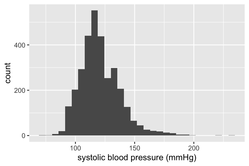
3. The distribution is roughly symmetric with a slight right skew, centered near 118–121 mmHg (median 118, mean 121). Most values fall between 110 and 130 mmHg (IQR = 20), with a standard deviation of about 17. There are a small number of high-end outliers extending to 232 mmHg.
t.test(nhanes$pulse, mu =72)
    One Sample t-test

data:  nhanes$pulse
t = 2.8235, df = 3178, p-value = 0.00478
alternative hypothesis: true mean is not equal to 72
95 percent confidence interval:
 72.18071 73.00205
sample estimates:
mean of x
 72.59138
4. The degrees of freedom equal \(n - 1 = 3178\), so there are \(n = 3179\) observations.
5. With 95% confidence, the mean resting pulse rate among U.S. adults is estimated to be between 72.18 and 73.00 bpm.
6. The data provide evidence that the mean resting pulse rate among U.S. adults differs from 72 bpm (T = 2.824 on 3178 degrees of freedom, p = 0.005).
Creativity and motivation
t.test(score ~ treatment, data = creativity, conf.level =0.99)
    Welch Two Sample t-test

data:  score by treatment
t = -2.9153, df = 43.108, p-value = 0.005618
alternative hypothesis: true difference in means between group Extrinsic and group Intrinsic is not equal to 0
99 percent confidence interval:
 -7.9749541 -0.3134517
sample estimates:
mean in group Extrinsic mean in group Intrinsic
               15.73913                19.88333
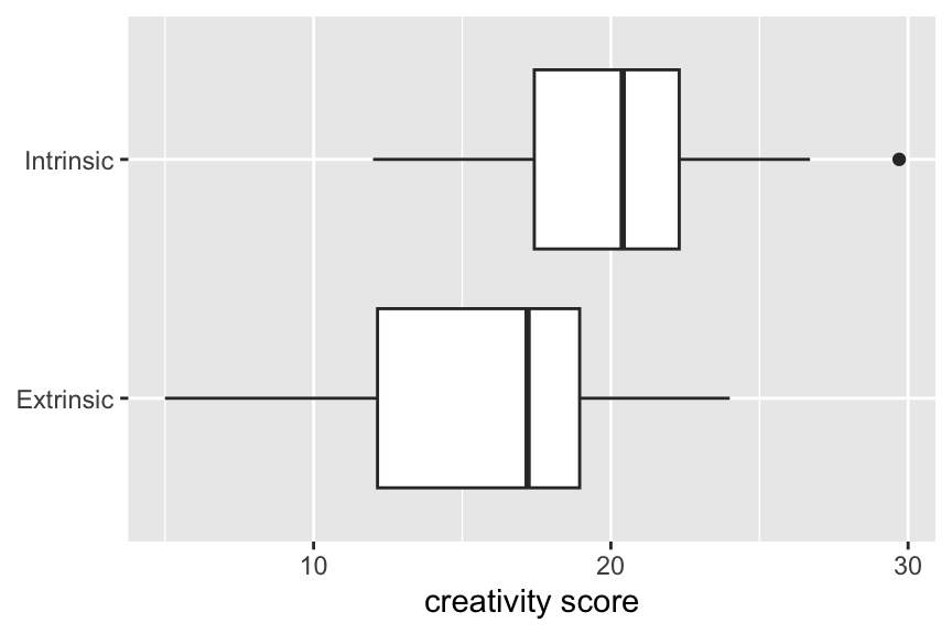
1. The assumptions seem plausible. Both distributions are roughly symmetric with no extreme outliers, and the group sizes (\(n = 24\) and \(n = 23\)) are sufficient. Because students were randomly assigned to groups, the independence assumption is satisfied.
2.\(H_0\colon \mu_\text{Intrinsic} = \mu_\text{Extrinsic}\) vs. \(H_A\colon \mu_\text{Intrinsic} \neq \mu_\text{Extrinsic}\)
3. The data provide evidence that intrinsic and extrinsic motivation produce different mean creativity scores (T = −2.915 on 43.11 degrees of freedom, p = 0.006).
4. The output reports the difference as \(\bar{x}_\text{Extrinsic} - \bar{x}_\text{Intrinsic}\). With 99% confidence, the mean creativity score under intrinsic motivation is estimated to be between 0.31 and 7.97 points higher than under extrinsic motivation.
5. The output does not report the SE directly. Reverse-engineer it from the \(t\) statistic using \(SE = \hat{\delta} / T\): \[SE = \frac{-4.14}{-2.915} \approx 1.42\] Then apply the empirical rule for an approximate 95% CI for the difference in means (\(\bar{x}_\text{Extrinsic} - \bar{x}_\text{Intrinsic}\)): \[-4.14 \pm 2(1.42) = -4.14 \pm 2.84 = (-6.98,\ -1.30)\]
Hippocampal volume
load('data/hippocampus.RData')t.test(hippocampus$affected - hippocampus$unaffected, mu =0, alternative ='less', conf.level =0.99)
    One Sample t-test

data:  hippocampus$affected - hippocampus$unaffected
t = -3.2289, df = 14, p-value = 0.003031
alternative hypothesis: true mean is less than 0
99 percent confidence interval:
        -Inf -0.03718909
sample estimates:
 mean of x
-0.1986667
1.\(H_0\colon \delta = 0\) vs. \(H_A\colon \delta < 0\), where \(\delta\) is the mean difference in left hippocampal volume (affected \(-\) unaffected).
2. The degrees of freedom equal \(n - 1 = 14\), so there are \(n = 15\) pairs of twins.
3. The data provide evidence that mean left hippocampal volume is smaller in twins affected by schizophrenia than in their unaffected co-twins (T = −3.229 on 14 degrees of freedom, p = 0.003).
4. With 99% confidence, the mean left hippocampal volume in affected twins is estimated to be at least 0.037 cm³ smaller than in their unaffected co-twins.
5.\(SE = 0.0615\) cm³. This estimates the variability of the sample mean difference \(\bar{d}\) across repeated samples of 15 twin pairs — in other words, how precisely \(\bar{d}\) estimates the true mean difference \(\delta\).
Mussel physiology
aov(aam.length ~ location, data = mussels)
Call:
   aov(formula = aam.length ~ location, data = mussels)

Terms:
                   location   Residuals
Sum of Squares  0.004519674 0.005394906
Deg. of Freedom           4          34

Residual standard error: 0.01259658
Estimated effects may be unbalanced
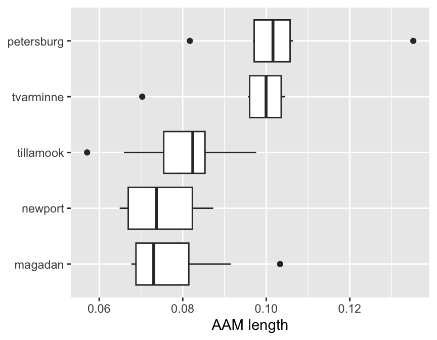
3. The data provide evidence of a difference in mean AAM length among the five mussel populations (F = 7.121 on 4 and 34 degrees of freedom, p < 0.001).
4.\(\eta^2 = SSG / SST = 0.004520 / 0.009915 = 0.456\). An estimated 45.6% of the variability in AAM length is attributable to differences among populations.