Applied Statistics for Life Sciences
Statistics and uncertainty
Life is full of uncertainty, and this can make a lot of questions hard to answer, because similar situations do not always result in the same outcome.
Statistical thinking: uncertainty (random variability) is measurable.
What statistics can offer:
- principles for designing studies and collecting data in order to capture outcome variability
- models that distinguish random from systematic variability
- methods for making robust inferences that account for uncertainty due to random/unexplained outcome variation
Course scope
The overarching goal of 218 is to introduce you to statistics in a hands-on way that is relevant to your major.
We will learn about statistical thinking and data analysis by studying classical methods (mostly developed 1900-1940) and their application to case studies from life sciences.
| Week | Topic(s) |
|---|---|
| 1 | Data semantics, descriptive statistics |
| 2-6 | Statistical inference for one or more population means |
| 7-8 | Statistical inference for population proportions from categorical data |
| 9-10 | Simple linear regression |
Most class meetings will be a mixture of lecture and lab activities.
Assessments
You will have three categories of graded assignments:
- homework (20%): 2-3 problems per class
- tests (60%): approximately every 3 weeks
- comprehensive final (20%): as scheduled by registrar
Select policies:
- one-hour grace period on all deadlines
- two free homework extensions (up to 1 week)
- one free homework exemption (or drop lowest score)
- test corrections will earn back a portion of missed credit
Grades
Outcome scores
Graded questions are matched to specific learning outcomes and you receive a per-outcome score, for example:
- L1: 58%
- L2: 83%
- L3: 77%
This means, roughly, you answered 58% of study design questions (L1) correctly.
(This is after accounting for assessment weighting and corrections.)
Letter grades
You must have at least 6 outcome scores over 50% to pass.
Your course grade is then determined by the number of outcome scores exceeding 80%:
| Grade | Number exceeding 80% |
|---|---|
| A | 9-10 |
| B | 6-8 |
| C | 3-5 |
| D | 0-2 |
Study design
What is a study?
A study is an effort to collect data in order to answer one or more research questions.
studies must be well-matched to research questions to provide good answers
how data are obtained is just as important as how the resulting data are analyzed
no analysis, no matter how sophisticated will rescue a poorly conceived study
A study unit is the smallest object or entity that is measured in a study; also called experimental unit or observational unit.
Sampling
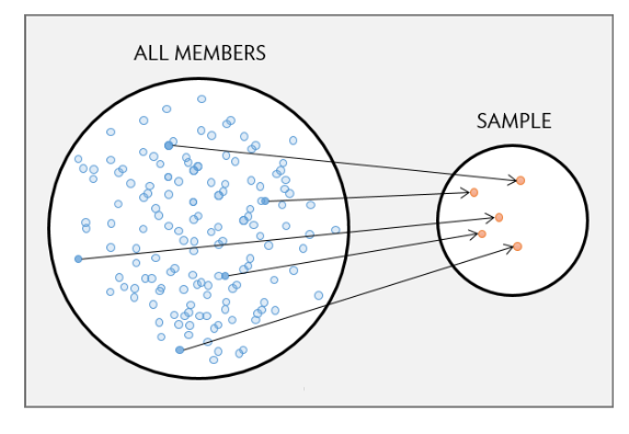
Study units should be chosen so as to represent a larger collection or “population”.

A study population is a collection of all study units of interest.
A sample is a subcollection:
- probability sample: all study units have some known “inclusion probability” or chance of being selected
- nonrandom/convenience sample: inclusion probabilities are not known
The gold standard is the simple random sample: all inclusion probabilities are equal.
- ensures samples of a fixed size from the population are exchangeable and thus “representative”
- justifies inferences about the population based on the sample
Two types of studies
Observational studies collect data from an existing situation without intervention.
Aim is to detect associations and patterns
Can’t be used to infer causal relationships owing to possible unmeasured confounding
Experiments collect data from a situation in which one or more interventions have been introduced by the investigator.
- Interventions are (supposed to be) randomized among study units
- Aim is to draw conclusions about the causal effect of interventions
- Stronger form of scientific evidence than an observational study
LEAP Study
Learning early about peanut allergy (LEAP) study:
640 infants in UK with eczema or egg allergy but no peanut allergy enrolled
each infant randomly assigned to peanut consumption and peanut avoidance groups
peanut consumption: fed 6g peanut protein daily until 5 years old
peanut avoidance: no peanut consumption until 5 years old
at 5 years old, oral food challenge (OFC) allergy test administered
13.3% of the avoidance group developed allergies, compared with 1.9% of the consumption group
Study characteristics
Study type: experiment
Study population: UK infants with eczema or egg allergy but no peanut allergy
Sample: 640 infants from population
Treatments: peanut consumption; peanut avoidance
Treatment allocation: completely randomized
Study outcome: development of peanut allergy by 5 years of age
Study results
Moderated peanut consumption causes a reduction in the likelihood of developing an allergy among infants with prior risk (eczema or egg allergies).
Why randomize?
Randomization eliminates confounding by ensuring that study interventions are independent of all extraneous conditions.
- no association is possible between study intervention and unobserved variables
- if outcomes differ systematically according to the intervention, you can be certain that the intervention is responsible
For example, imagine an observational version of the LEAP study in which allergy rates are compared between children who consumed peanuts as infants and those who didn’t.
- those with reactions are more likely to become avoiders
- could inflate the observed difference relative to the true effect
Randomizing consumption regimens eliminates this possibility.
Data semantics
Data semantics
Data are a set of measurements.
A variable is any measured attribute of study units.
An observation is a measurement of one or more variables taken on one particular study unit.
It is usually expedient to arrange data values in a table in which each row is an observation and each column is a variable:

LEAP example
A table showing the observations and variables for the LEAP study would look like this:
| participant.ID | treatment.group | ofc.test.result |
|---|---|---|
| LEAP_100522 | Peanut Consumption | PASS OFC |
| LEAP_103358 | Peanut Consumption | PASS OFC |
| LEAP_105069 | Peanut Avoidance | PASS OFC |
| LEAP_105328 | Peanut Consumption | PASS OFC |
The table you saw in the reading was a summary of the data (not the data itself):
| FAIL OFC | PASS OFC | |
|---|---|---|
| Peanut Avoidance | 36 | 227 |
| Peanut Consumption | 5 | 262 |
Numeric and categorical variables
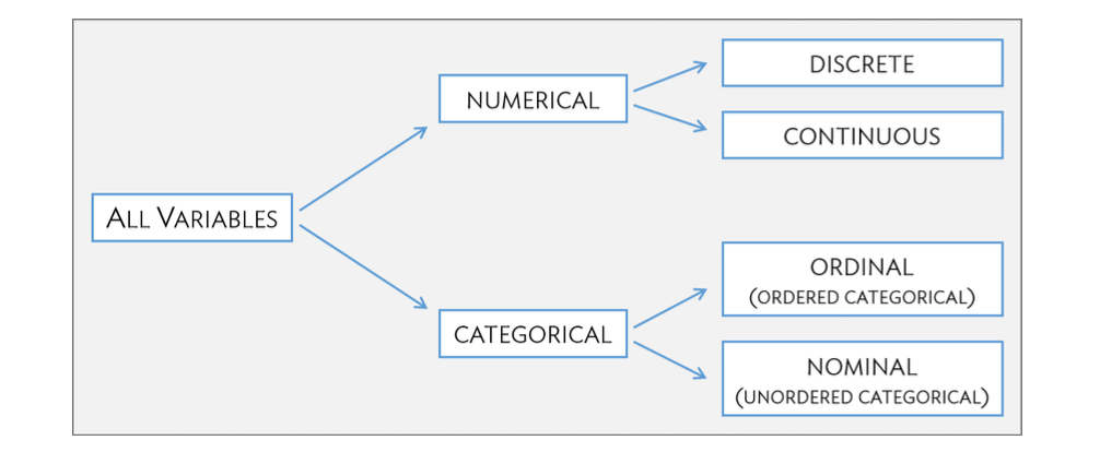
Variables are classified according to their values. Values can be one of two different types:
- A variable is numeric if its value is a number
- A variable is categorical if its value is a category, usually recorded as a name or label
For example:
- the value of
sexcan be male or female, so it is categorical - whereas
age(in years) can be any positive integer, so it is numeric
Variable subtypes
Further distinctions are made based on the type of number or type of category used to measure an attribute. Can you match the subtypes to the variables at right?

| age | hispanic | grade | weight |
|---|---|---|---|
| 15 | not | 10 | 78.02 |
| 18 | hispanic | 12 | 78.47 |
| 17 | not | 11 | 95.26 |
| 18 | not | 12 | 95.26 |
- a numerical variable is discrete if there are ‘gaps’ between its possible values
- a numerical variable is continuous if there are no such gaps
- a categorical variable is nominal if its levels are not ordered
- a categorical variable is ordinal if its levels are ordered
Many ways to measure attributes
Variable type (or subtype) is not an inherent quality — attributes can often be measured in many different ways.
For instance, age might be measured as either a discrete, continuous, or ordinal variable, depending on the situation:
| Age (years) | Age (minutes) | Age (brackets) |
|---|---|---|
| 12 | 6307518.45 | 10-18 |
| 8 | 4209187.18 | 5-10 |
| 21 | 11258103.08 | 18-30 |
Numeric variables can always be discretized into categorical variables.
Your turn
Classify each variable as nominal, ordinal, discrete, or continuous:
| ndrm.ch | genotype | sex | age | race | bmi |
|---|---|---|---|---|---|
| 33.3 | CT | Female | 19 | Caucasian | 21.01 |
| 71.4 | CT | Female | 18 | Other | 23.18 |
| 37.5 | CC | Female | 21 | Caucasian | 28.92 |
| 50 | CC | Female | 28 | Asian | 21.16 |
Data are from an observational study investigating demographic, physiological, and genetic characteristics associated with muscle strength.
ndrm.chis change in strength in nondominant arm after resistance traininggenotypeindicates genotype at a particular location within the ACTN3 gene
Data summaries
Summary statistics
A statistic is, mathematically, a function of the values of two or more observations
For numeric variables, the most common summary statistic is the average value:
average=sum of values# observations
For example, the average percent change in nondominant arm strength was 53.291%.
For categorical variables, the most common summary statistic is a proportion:
proportioni=# observations in category i# observations
For example:
| CC | CT | TT |
|---|---|---|
| 0.2908 | 0.4387 | 0.2706 |
Mathematical notation
Typically, a set of observations is written as:
x1,x2,…,xn
- x represents the variable (e.g., genotype, age, percent change, etc.)
- i (subscript) Indexes observations: xi is the ith observation
- n is the total Number of observations
The sum of the observations is written ∑ixi, where the symbol ∑ stands for ‘summation’. This is useful for writing the formula for computing an average:
ˉx=1nn∑i=1xi(average=1# observations×sum of values)
Descriptive analyses
Sometimes, a few clever summary statistics can be used to answer a research question.
How much does the average change in arm strength differ by genotype among participants, if at all?
Computing per-genotype group averages provides an answer:
| genotype | avg.change | n.obs | prop.obs |
|---|---|---|---|
| TT | 58.08 | 161 | 0.2706 |
| CT | 53.25 | 261 | 0.4387 |
| CC | 48.89 | 173 | 0.2908 |
Number of observations and proportions are included because they provide information about genotype frequencies in the sample.
- conveys how many individuals were measured
- also provides an estimate of genotype frequencies in the population
Statistical inference
Data summaries indicated that the average change was highest (58.05% increase) among individuals with genotype TT.
This is a descriptive finding: it’s a fact about individuals in the study.
Can we conclude that the same is true of all individuals, including those not in the study?
- not with absolute certainty, but…
- if the sample was representative of a broader population, we can make inferences with certain statistical guarantees on the error probability
- how big of a gap do we need to see to be confident that there are true differences in response to strength training associated with genotype?
Statistical inference refers to drawing conclusions about a population from a sample while accounting for uncertainty, and is the focus of this course.
STAT218