STAT218 - Confidence intervals

Today’s agenda

[lecture] confidence intervals for the mean
[lab] computing and interpreting confidence intervals

From last time

Under simple random sampling:

the sample mean provides a good point estimate of the population mean
its estimated sampling variability is given by the standard error

mean	sd	n	se
5.043	1.075	3179	0.01906

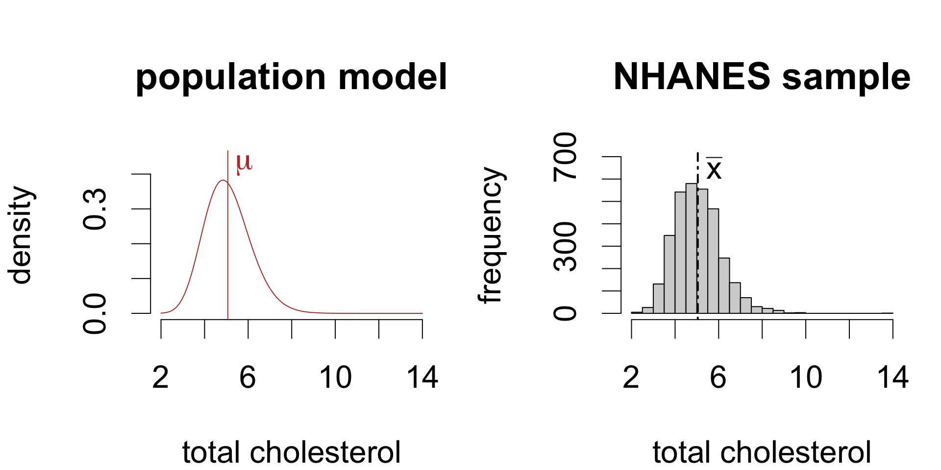
The mean total HDL cholesterol among the U.S. adult population is estimated to be 5.043 mmol/L (SE 0.0191).

Interval estimation

A common interval estimate for the population mean is:

The mean total cholesterol among U.S. adults is estimated to be between 5.005 and 5.081 mmol/L.

Two related questions:

In what sense are these values “plausible”?
Where did the number 2 come from?

The model

Consider the statistic:

The sampling distribution of is well-approximated by a model whenever either:

the population distribution is symmetric and unimodal

OR

the sample size is not too small

model interpretation

The area under the density curve between any two values gives the proportion of random samples for which .

For example:

for 50% of samples,

# area less than 0
pt(0, df = 20 - 1)

[1] 0.5

written as

model interpretation

The area under the density curve between any two values gives the proportion of random samples for which .

For example:

for 83.5% of samples,

# area less than 1
pt(1, df = 20 - 1)

[1] 0.8350616

written as

model interpretation

The area under the density curve between any two values gives the proportion of random samples for which .

For example:

for 97% of samples,

# area less than 2
pt(2, df = 20 - 1)

[1] 0.969999

written as

model interpretation

The area under the density curve between any two values gives the proportion of random samples for which .

For example:

for 3% of samples,

# area greater than 2
pt(2, df = 20 - 1, lower.tail = F)

[1] 0.03000102

notice:

model interpretation

The area under the density curve between any two values gives the proportion of random samples for which .

For example:

for 13.5% of samples,

# area between 1 and 2
pt(2, df = 20 - 1) - pt(1, df = 20 - 1)

[1] 0.1349374

notice:

model interpretation

The area under the density curve between any two values gives the proportion of random samples for which .

For example:

for 94% of samples,

# area between 1 and 2
pt(2, df = 20 - 1) - pt(-2, df = 20 - 1)

[1] 0.939998

written

A closer look at interval construction

So where did that 2 come from in the margin of error for our interval estimate?

Well:

For 94% of all random samples, the interval covers the population mean.

So the number 2 determines the proportion of samples for which the interval covers the mean, known as its coverage.

Effect of sample size

The sample size determines the exact shape of the model through its ‘degrees of freedom’ . This changes the areas slightly.

The exact coverage quickly converges to just over 95% as the sample size increases.

n	coverage
4	0.8607
8	0.9144
16	0.9361
32	0.9457
64	0.9502
128	0.9524
256	0.9534

Changing the coverage

Consider a slightly more general expression for an interval for the mean:

The number is called a critical value. It determines the coverage.

larger higher coverage
smaller lower coverage

The so-called “empirical rule” is that:

approximately 68% coverage
approximately 95% coverage
approximately 99.7% coverage

Interpreting critical values

Look at how the areas add up so that: Moreover:

So the critical value 2 is actually the 97th percentile of the sampling distribution of .

also called the 0.97 “quantile”
(percentiles expressed in proportions are called quantiles)

Exact coverage using quantiles

To engineer an interval with a specific coverage, use the th quantile where:

In R:

# coverage 95% using t quantile
coverage <- 0.95
q.val <- 1 - (1 - coverage)/2
crit.val <- qt(q.val, df = 20 - 1)
crit.val

[1] 2.093024

The effect of increasing/decreasing coverage on the quantile is:

increase coverage larger quantile wider interval
decrease coverage smaller quantile narrower interval

Coverage vs. precision

Precision refers to how wide or narrow the interval is.

Precision depends on every component of the margin of error:

critical value used
sample size
variability of values

By contrast, coverage depends only on the critical value used.

Confidence intervals

Interval estimates constructed to achieve a specified coverage are called “confidence intervals”; the coverage is interpreted and reported as a “confidence level”.

# ingredients
cholesterol.mean <- mean(cholesterol)
cholesterol.sd <- sd(cholesterol)
cholesterol.n <- length(cholesterol)
cholesterol.se <- cholesterol.sd/sqrt(cholesterol.n)
crit.val <- qt(1 - (1 - 0.95)/2, df = cholesterol.n - 1)

# interval
cholesterol.mean + c(-1, 1)*crit.val*cholesterol.se

[1] 5.005566 5.080310

With 95% confidence, the mean total cholesterol among U.S. adults is estimated to be between 5.0056 and 5.0803 mmol/L.

The general formula for a confidence interval for the population mean is

where is a critical value, obtained as a quantile of the model and chosen to ensure a specific coverage.

Recap

The “common” interval estimate for the mean is actually an approximate 95% confidence interval:

captures the population mean for roughly 95% of random samples
replacing 2 with a quantile allows the analyst to adjust coverage
the model is an approximation for the sampling distribution of
- approximation improves with increasing sample size or symmetry
- usually good quality except in “extreme” situations

Interval interpretation:

With [XX]% confidence, the mean [population parameter] is estimated to be between [lower bound] and [upper bound] [units].

Confidence intervals

Today’s agenda

From last time

Interval estimation

The model

model interpretation

model interpretation

model interpretation

model interpretation

model interpretation

model interpretation

A closer look at interval construction

Effect of sample size

Changing the coverage

Interpreting critical values

Exact coverage using quantiles

Coverage vs. precision

Confidence intervals

Recap

Extras

Simulation of coverage