Foundations for statistical inference
Point estimation and sampling variability
Today’s agenda
- [lecture] point estimation and sampling variability
- [lab] calculating point and interval estimates
- [activity] estimating the class’ mean arm span
Point estimation
Population distributions
A population distribution is a frequency distribution across all possible study units.
For simple random samples, the observed distribution of sample values resembles the population distribution:
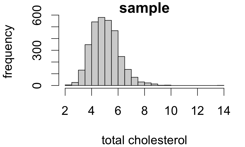
The larger the sample, the closer the resemblance.1
Foundations for inference
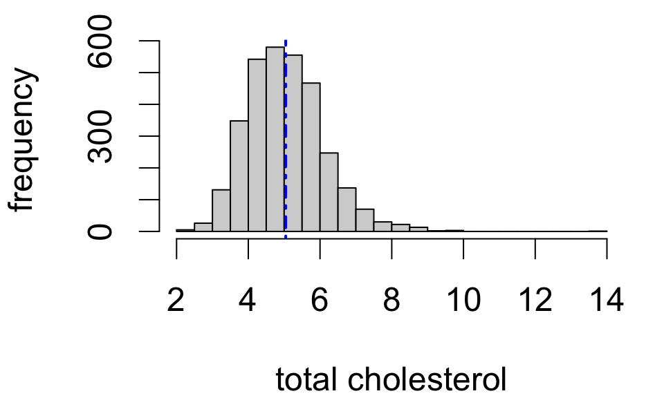
Population statistics are called parameters. These are fixed but unknown values.
| Population mean | Population SD |
|---|---|
| 5.067 | 1.126 |

Notation:
- population mean μ
- population standard deviation σ
Foundations for inference
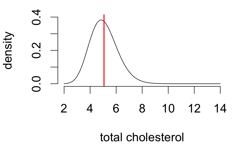
Sample statistics provide point estimates of the corresponding population statistics.
Notation:
- sample mean ˉx
- sample standard deviation sx
| Sample mean | Sample SD | Sample size |
|---|---|---|
| 5.043 | 1.075 | 3179 |
Foundations for inference
| Population mean | Population SD |
|---|---|
| 5.067 | 1.126 |
| Sample mean | Sample SD | Sample size |
|---|---|---|
| 5.043 | 1.075 | 3179 |

So we might say: “mean total cholesterol in the study population is estimated to be 5.043”
A difficulty
Different samples yield different estimates.
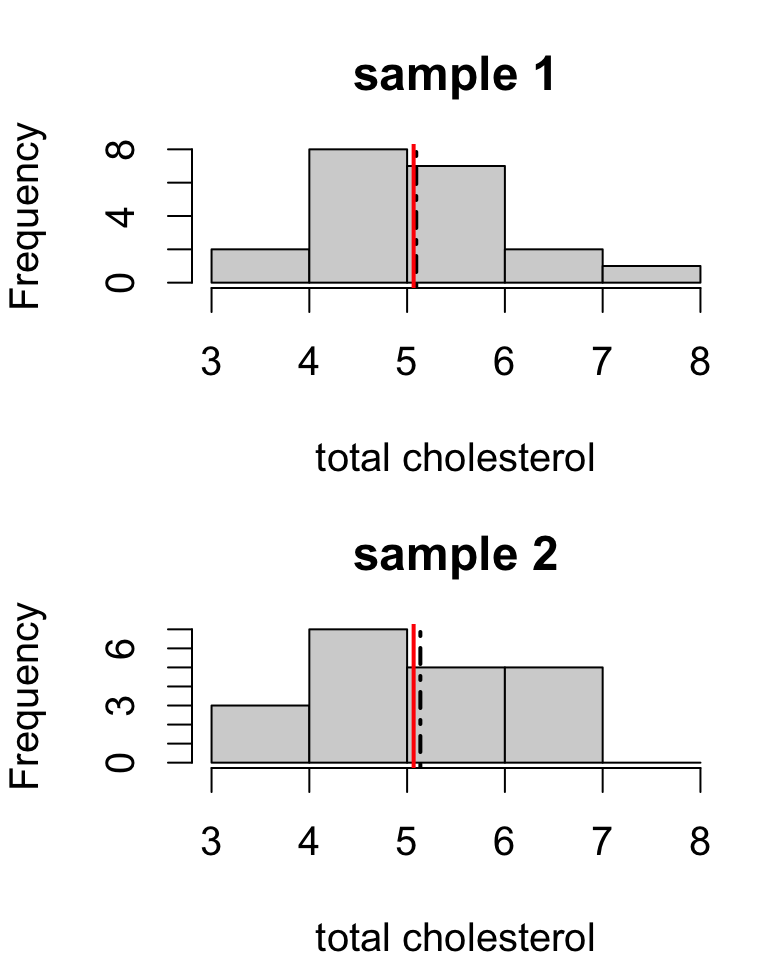
Sample means:
| sample.1 | sample.2 |
|---|---|
| 5.093 | 5.136 |
- estimates are close but not identical
- the population mean can’t be both 5.093 and 5.136
- probably neither estimate is exactly correct
- but both estimates should have similar errors if the study design is identical between the two samples
Simulating sampling variability
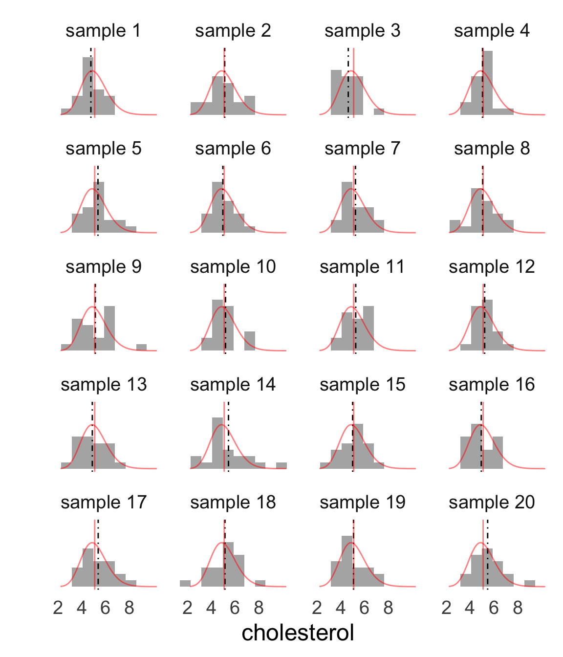
These are 20 random samples with the sample mean indicated by the dashed line and the population distribution and mean overlaid in red.
- sample size n=20
- frequency distributions differ a lot
- sample means differ some
We can actually measure this variability!
Simulating sampling variability
If we had means calculated from a much larger number of samples, we could make a frequency distribution for the values of the sample mean.
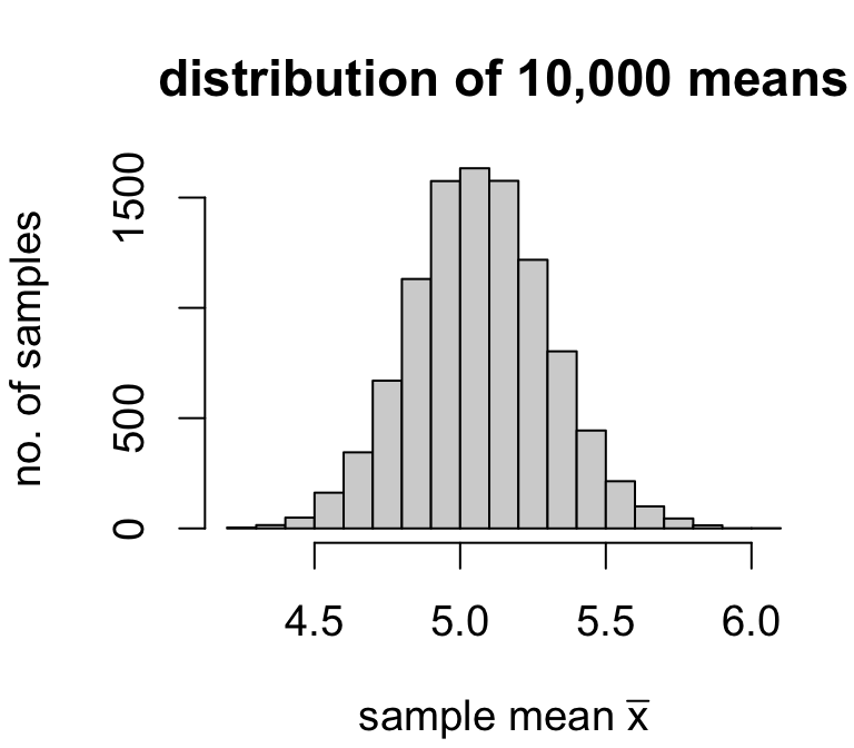
| sample | 1 | 2 | ⋯ | 10,000 |
| mean | 4.957 | 5.039 | ⋯ | 5.24 |
We could then use the usual measures of center and spread to characterize the distribution of sample means.
- mean of ˉx: 5.068425
- standard deviation of ˉx: 0.2369404
Across 10,000 random samples of size 20, the average estimate was 5.07 and the variability of estimates was 0.237.
Sampling distributions
What we are simulating is known as a sampling distribution: the frequency of values of a statistic across all possible random samples.
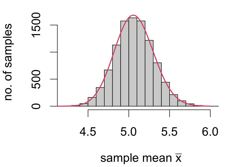
When data are from a random sample, statistical theory provides that the sample mean ˉx has a sampling distribution with
- mean μ (population mean)
- standard deviation σ√n(population SD√sample size)
regardless of the population distribution.
In other words, across all random samples of a fixed size…
- [accuracy] on average, the sample mean equals the population mean
- [precision] on average, the estimation error is σ√n
Measuring sampling variability
In practice we use an estimate of sampling variability known as a standard error: SE(ˉx)=sx√n(sample SD√sample size)
For example:
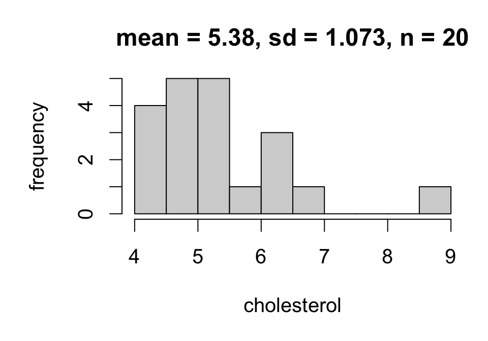
SE(ˉx)=1.073√20=0.240
Reporting point estimates
It is common style to report the value of a point estimate with a standard error given parenthetically.
Statistics from full NHANES sample:
| mean | sd | n |
|---|---|---|
| 5.043 | 1.075 | 3179 |
The mean total cholesterol among the population is estimated to be 5.043 mmol/L (SE 0.019)
This style of report communicates:
- parameter of interest
- value of point estimate
- error/variability of point estimate
Sources of variability
There are two potential sources of variability in estimates:
- population variability (σ)
- sampling variability (determined by n)
For example, the estimates below are equally precise:
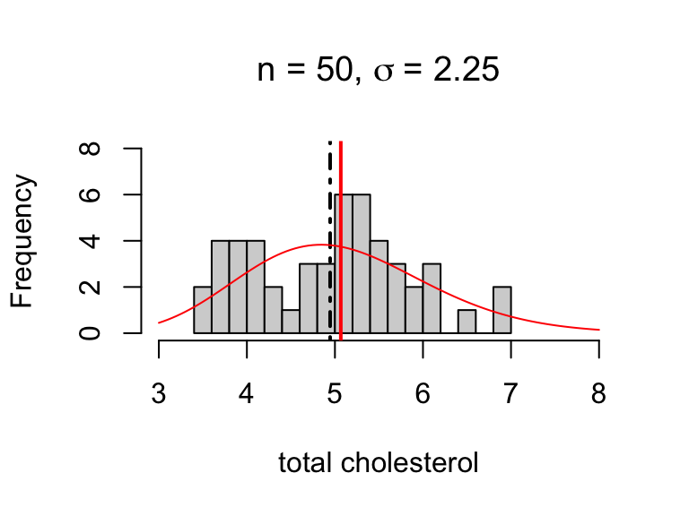
SE(ˉx) = 0.1265079
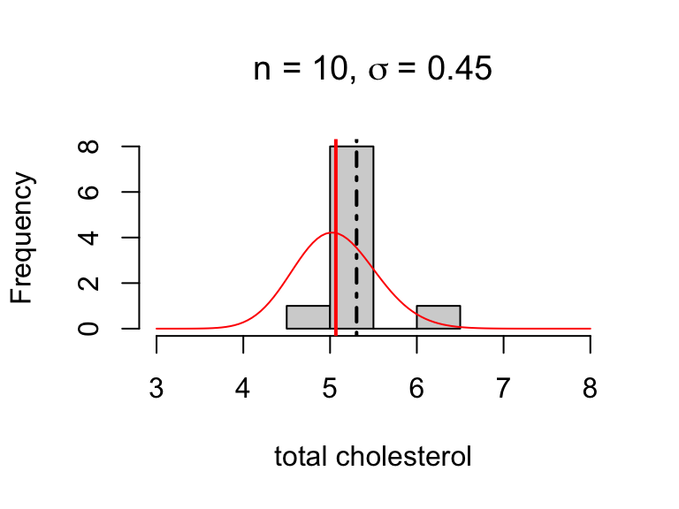
SE(ˉx) = 0.1223712
Interval estimation
Interval estimation
An interval estimate is a range of plausible values for a population parameter.
The general form of an interval estimate is
point estimate±margin of error
where the “margin of error” reflects the sampling variability.
- more sampling variability ⟹ larger margin of error
- less sampling variability ⟹ smaller margin of error
An interval for the mean
A common interval for the population mean is: ˉx±2×SE(ˉx)whereSE(ˉx)=(sx√n)
By hand: 5.043±2×0.0191=(5.005,5.081)
Interpretation: the mean total cholesterol among the study population is estimated to be between 5.005 and 5.081 mmol/L.
Questions for next time
- In what sense are the values in the interval estimate “plausible”?
- Why use 2×SE(ˉx) for the margin of error?
- What do you expect would happen if the margin of error were 3×SE(ˉx)?
STAT218