| mean | sd | n | se |
|---|---|---|---|
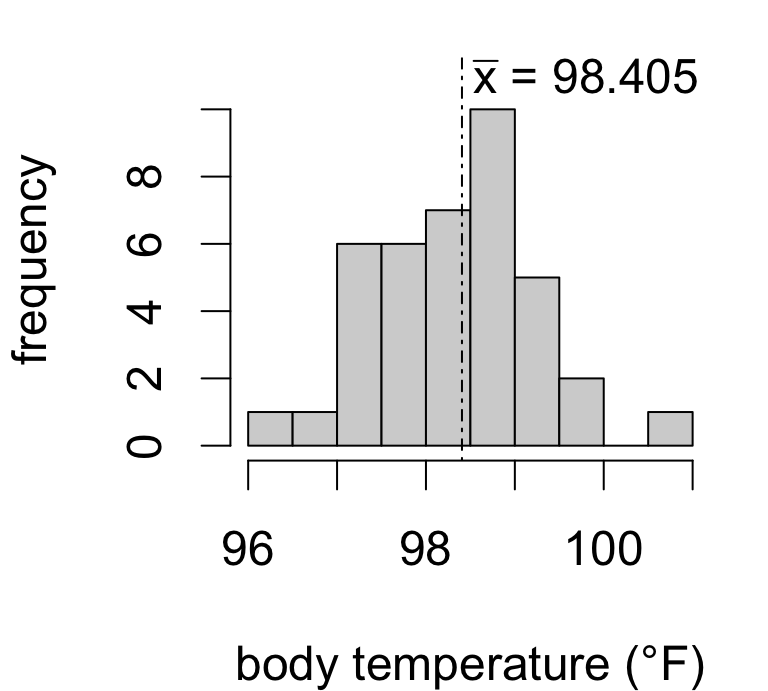
| 98.41 | 0.9162 | 39 | 0.1467 |
One sample inference for a population mean
t.test()
| mean | sd | n | se |
|---|---|---|---|
| 98.41 | 0.9162 | 39 | 0.1467 |
Is the true mean body temperature actually 98.6°F?
Seems plausible given our data.
But what if the sample mean were instead…
| ˉx | consistent with μ=98.6? |
|---|---|
| 98.30 | probably still yes |
| 98.15 | maybe |
| 98.00 | hesitating |
| 97.85 | skeptical |
| 97.40 | unlikely |
Consider how many standard errors away from the hypothesized value we’d be:
| ˉx | estimation error | no. SE’s | interpretation |
|---|---|---|---|
| 98.30 | -0.3 | 2 | double the average error |
| 98.15 | -0.45 | 3 | triple the average error |
| 98.00 | -0.6 | 4 | quadruple |
| 97.85 | -0.75 | 5 | quintuple |
| 97.40 | -1.2 | 8 | octuple! |
We know from interval coverage that:
So if the estimation error exceeds 2-3SE, the data aren’t consistent with the hypothesis.
If we want to test the hypothesis
H0:μ=98.6
against the alternative
HA:μ≠98.6
then we consider the test statistic
T=ˉx−98.6sx/√n(estimation errorstandard error)
Two possible outcomes:
estimation error is small relative to standard error
⟹ the data are consistent with H0
estimation error is large relative to standard error
⟹ the data favor HA over H0
To formalize the test we just need to decide: how many SE’s is large enough to reject H0?
If the population mean is in fact 98.6°F then T=ˉx−98.6sx/√n(estimation errorstandard error) has a sampling distribution that is well-approximated by a t39−1 model.

If the population mean is in fact 98.6°F then T=ˉx−98.6sx/√n(estimation errorstandard error) has a sampling distribution that is well-approximated by a t39−1 model.

If the population mean is in fact 98.6°F then T=ˉx−98.6sx/√n(estimation errorstandard error) has a sampling distribution that is well-approximated by a t39−1 model.

If the population mean is in fact 98.6°F then T=ˉx−98.6sx/√n(estimation errorstandard error) has a sampling distribution that is well-approximated by a t39−1 model.

If the population mean is in fact 98.6°F then T=ˉx−98.6sx/√n(estimation errorstandard error) has a sampling distribution that is well-approximated by a t39−1 model.

P(|T|>1.328)=0.192
If the hypothesis were true, we’d see at least as much (absolute) estimation error 19.2% of the time. So the data are consistent with the hypothesis μ=98.6.
If the population mean is in fact 98.6°F then T=ˉx−98.6sx/√n(estimation errorstandard error) has a sampling distribution that is well-approximated by a t39−1 model.

P(|T|>2.726)=0.0096
If the hypothesis were true, we’d see at least as much estimation error only 0.96% of the time. So the data are not consistent with the hypothesis μ=98.6
We just made these assessments:
| sample.mean | se | t.stat | how.often | evaluation |
|---|---|---|---|---|
| 98.41 | 0.1467 | -1.328 | 0.192 | not unusual |
| 98.2 | 0.1467 | -2.726 | 0.009632 | unusual |
The sampling frequency we’re calculating above is called a p-value: the proportion of samples for which the test statistic, under H0, would exceed the observed value.
The convention is to reject the hypothesis whenever p < 0.05.
| sample.mean | se | t.stat | how.often |
|---|---|---|---|
| 98.41 | 0.1467 | -1.328 | 0.192 |
| 98.2 | 0.1467 | -2.726 | 0.009632 |
Suppose we decided to reject H0 whenever p<0.2 so that both outcomes above were considered unusual. Then if in fact μ=98.6:
So the level of the test is an error rate: how often the test is expected to falsely reject H0.
To test the hypotheses:
{H0:μ=μ0HA:μ≠μ0
Steps:
# point estimate and standard error
temp.mean <- mean(temps$body.temp)
temp.mean.se <- sd(temps$body.temp)/sqrt(nrow(temps))

# compute test statistic
tstat <- (temp.mean - 98.6)/temp.mean.se
tstat
[1] -1.328265# proportion of samples where T exceeds observed value
p.val <- 2*pt(abs(tstat), df = 38, lower.tail = F)
p.val[1] 0.1920133[1] FALSEWe call this a t-test for the population mean. Conventional summary interpretation:
The data do not provide evidence that the mean body temperature differs from 98.6°F (T = -1.328 on 38 degrees of freedom, p = 0.192).
There are two possible findings for a test:
A reject decision is interpreted as:
The data provide evidence that… [against H0/favoring HA]
A fail to reject decision is interpreted as:
The data do not provide evidence that… [against H0/favoring HA]
There are two ways to make a mistake in a hypothesis test – two “error types”.
| Reject H0 | Fail to reject H0 | |
|---|---|---|
| True H0 | type I error | correct decision |
| False H0 | correct decision | type II error |
Any statistical test will have certain error rates:
The t-test for the mean test controls the type I error rate at level α.
Type II error is trickier, because the sampling distribution of the test statistic depends on the (unknown) population mean – we’ll revisit this later.
A hypothesis test boils down to deciding whether your estimate is too far from a hypothetical value for that hypothesis to be plausible.
To test the hypotheses:
{H0:μ=μ0HA:μ≠μ0
We use the test statistic:
T=ˉx−μ0SE(ˉx)(estimation error under H0standard error)
We say H0 is implausible at level α if:
This decision rule controls the type I error rate at level α.
Test the hypothesis that the average U.S. adult sleeps 8 hours.

| estimate | std.err | tstat | pval |
|---|---|---|---|
| 6.96 | 0.02 | -42.53 | <0.0001 |
95% confidence interval: (6.91, 7.01)
The data provide evidence that the average U.S. adult does not sleep 8 hours per night (T = -42.53 on 3178 degrees of freedom, p < 0.0001). With 95% confidence, the mean nightly hours of sleep among U.S. adults is estimated to be between 6.91 and 7.01 hours, with a point estimate of 6.59 hours (SE: 0.0245).
The test and interval convey complementary information:
A level α test rejects H0:μ=μ0 exactly when μ0 is outside the (1−α)×100% confidence interval for μ.

Left, p-values for a sequence of tests:
In other words:
level α test rejects⟺1−α CI excludes
t.test(...) functionSince tests and intervals go together, there is a single R function that computes both.
You have to make the decision using the p value:
Take a moment to locate each component of the test and estimates from the output.
Does the average U.S. adult sleep less than 7 hours?
This example leads to a lower-sided alternative:
{H0:μ=7HA:μ<7
The test statistic is the same as before:
T=ˉx−7SE(ˉx)=−1.671
The lower-sided p-value is 0.0474:

For the p-value, we look at how often T is larger in the direction of the alternative.
Does the average U.S. adult sleep more than 7 hours?*
Now the alternative is in the opposite direction:
{H0:μ=7HA:μ>7
The test statistic is the same as before:
T=ˉx−7SE(ˉx)=−1.671
The upper-sided p-value is 0.9526:

For the p-value, we look at how often T is larger in the direction of the alternative.
Tests for the mean can involve directional or non-directional alternatives. We refer to these as one-sided and two-sided tests, respectively.
| Test type | Alternative | Direction favoring alternative |
|---|---|---|
| Upper-sided | μ>μ0 | larger T |
| Lower-sided | μ<μ0 | smaller T |
| Two-sided | μ≠μ0 | larger |T| |
The direction of the test affects the p-value calculation (and thus decision), but won’t change the test statistic.
Conceptually tricky, but easy in R:
Do U.S. adults sleep 7 hours per night?
Do U.S. adults sleep less than 7 hours per night?
Do U.S. adults sleep more than 7 hours per night?
Your turn:
    One Sample t-test

data:  sleep
t = -1.671, df = 3178, p-value = 0.09482
alternative hypothesis: true mean is not equal to 7
95 percent confidence interval:
 6.911123 7.007090
sample estimates:
mean of x
 6.959107
    One Sample t-test

data:  sleep
t = -1.671, df = 3178, p-value = 0.04741
alternative hypothesis: true mean is less than 7
95 percent confidence interval:
     -Inf 6.999372
sample estimates:
mean of x
6.959107 The tests don’t agree if the same level is used.
Consider: a type I error occurs in each case if…
Using level α=0.05 for both tests means that falsely inferring μ<7 occurs:
So test (B) is more sensitive to data suggesting μ<7 because it permits errors at a higher rate.
STAT218