    Welch Two Sample t-test

data:  rainfall by treatment
t = 1.9982, df = 33.855, p-value = 0.02689
alternative hypothesis: true difference in means between group seeded and group unseeded is greater than 0
95 percent confidence interval:
 42.63408      Inf
sample estimates:
  mean in group seeded mean in group unseeded
441.9846 164.5885 Analysis of Variance
Inference comparing multiple population means
Today’s agenda
- [lecture] statistical power
- [lecture] omnibus F test for the one-way ANOVA model
- [lab] fitting ANOVA models in R
Statistical power
p-values and type I errors
A p-value captures how often you’d make a mistake if H0 were true.
If there is no effect of cloud seeding, then we would see T>1.9982 for 2.69% of samples.
While unlikely, our sample could have been among that 2.69%
By rejecting here we are willing to be wrong 2.69% of the time
Type II errors
But you can also make a mistake when H0 is false!
    Welch Two Sample t-test

data:  rainfall by treatment
t = 1.9982, df = 33.855, p-value = 0.02689
alternative hypothesis: true difference in means between group seeded and group unseeded is greater than 0
95 percent confidence interval:
 42.63408      Inf
sample estimates:
  mean in group seeded mean in group unseeded
              441.9846               164.5885
Suppose we test at the 1% level.
The test fails to reject (p>0.01), but that doesn’t completely rule out HA.
The estimated effect – an increase of 277.4 acre-feet – could be too small relative to the variability in rainfall.
Simulating type II errors
Summary stats for cloud data:
| treatment | mean | sd | n |
|---|---|---|---|
| seeded | 442 | 650.8 | 26 |
| unseeded | 164.6 | 278.4 | 26 |
We can approximate the type II error rate by:
- simulating datasets with matching statistics
- performing upper-sided tests of no difference
- computing the proportion of fail-to-reject decisions
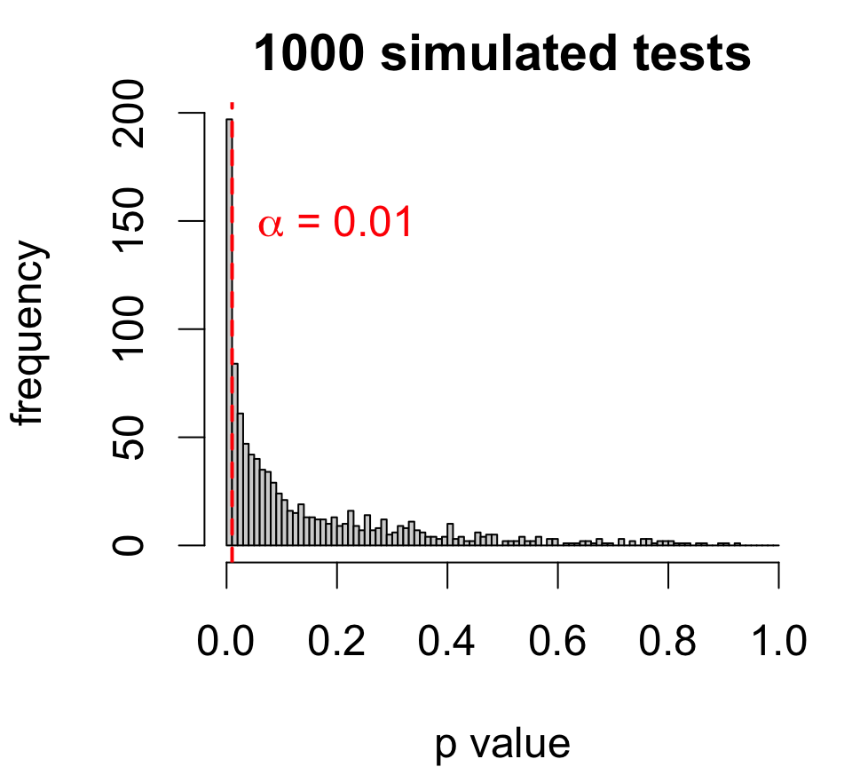
If in fact the effect size is exactly 277, a level 1% test with similar data will fail to reject 80.3% of the time!
Larger effect size
Summary stats for cloud data:
| treatment | mean | sd | n |
|---|---|---|---|
| seeded | 442 | 650.8 | 26 |
| unseeded | 164.6 | 278.4 | 26 |
Type II error rate depends on effect size:
- larger effect ⟶ lower error rate

If in fact the effect size is exactly 400, a level 1% test with similar data will fail to reject 57.9% of the time.
Smaller effect size
Summary stats for cloud data:
| treatment | mean | sd | n |
|---|---|---|---|
| seeded | 442 | 650.8 | 26 |
| unseeded | 164.6 | 278.4 | 26 |
Type II error rate depends on effect size:
- larger effect ⟶ lower error rate
- smaller effect ⟶ higher error rate
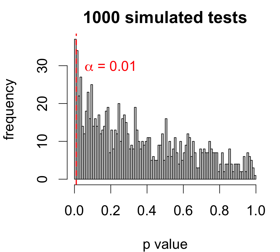
If in fact the effect size is exactly 100, a level 1% test with similar data will fail to reject 96.3% of the time.
Statistical power
The power of a test refers to its true rejection rate under an alternative and is defined as: β=(1−type II error rate)⏟correct decision rate when alternative is true
Power is often interpreted as a detection rate:
- high type II error ⟶ low power ⟶ low detection rate
- low type II error ⟶ high power ⟶ high detection rate
Power depends on the exact alternative scenario:
- low for alternatives close to the hypothetical value (e.g., δ0=0)
- high for alternatives far from the hypothetical value (e.g., δ0=0)
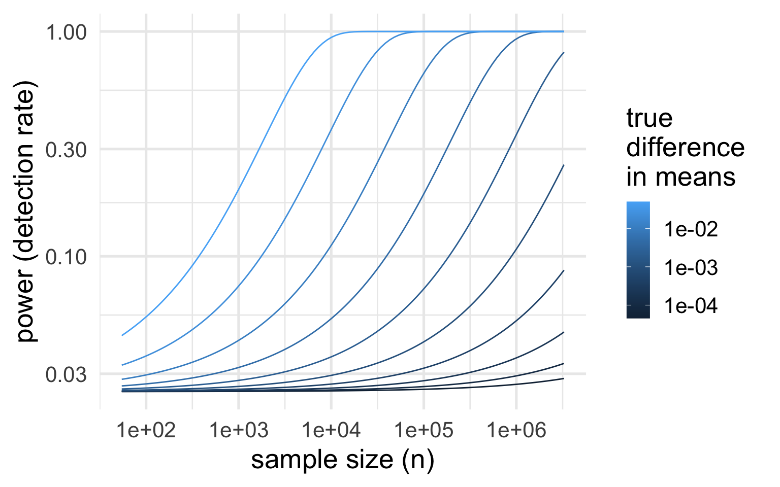
Power curves
Power is usually represented as a curve depending on the true difference.
Power curves for the test applied to the cloud data:

Assumptions:
- significance level α=0.05
- population standard deviation σ=650 (larger of two group estimates)
Which sample size achieves a specific β,δ?
Sample size calculation
If you were (re)designing the study, how much data should you collect to detect a specified effect size?
To detect a difference of 250 or more due to cloud seeding with power 0.9:
power.t.test(power = 0.9, # target power level
             delta = 250, # smallest difference
             sd = 650, # largest population SD
             sig.level = 0.01,
             type = 'two.sample',
             alternative = 'one.sided')
     Two-sample t test power calculation

              n = 177.349
          delta = 250
             sd = 650
      sig.level = 0.01
          power = 0.9
    alternative = one.sided

NOTE: n is number in *each* group
For a conservative estimate, use:
- overestimate of the larger of the two standard deviations
- minimum difference of interest
⟹ we need at least 177 observations in each group to detect a difference of 250 or more at least 90% of the time
Revisiting body temperatures
Does mean body temperature differ between men and women?
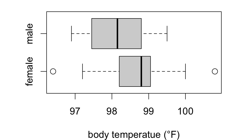
Test H0:μF=μM against HA:μF≠μM
    Welch Two Sample t-test

data:  body.temp by sex
t = 1.7118, df = 34.329, p-value = 0.09595
alternative hypothesis: true difference in means between group female and group male is not equal to 0
95 percent confidence interval:
 -0.09204497  1.07783444
sample estimates:
mean in group female   mean in group male
            98.65789             98.16500
Suggestive but insufficient evidence that mean body temperature differs by sex.
Notice: estimated difference (F - M) is 0.493 °F (SE 0.2879)
What if we had more data?
Here are estimates from two larger samples of 65 individuals each (compared with 19, 20):
| sex | mean.temp | se | n |
|---|---|---|---|
| female | 98.39 | 0.09222 | 65 |
| male | 98.1 | 0.08667 | 65 |
- estimated difference (F - M) is smaller 0.2892 °F
- but so is the standard error SE 0.1266 (recall more data ⟷ better precision)
    Welch Two Sample t-test

data:  body.temp by sex
t = 2.2854, df = 127.51, p-value = 0.02394
alternative hypothesis: true difference in means between group female and group male is not equal to 0
95 percent confidence interval:
 0.03881298 0.53964856
sample estimates:
mean in group female   mean in group male
            98.39385             98.10462
The data provide evidence that mean body temperature differs by sex (T = 2.29 on 127.51 degrees of freedom, p = 0.02394).
A statistical trap
If you collect enough data, you can detect an arbitrarily small difference in means.
So keep in mind:
- statistical significance ≠ practical significance
- large samples will tend to produce statistically significant results
It’s a good idea to always check your point estimates and ask whether findings are practically meaningful.
ANOVA
Chick weight data
Chick weights at 20 days of age by diet:

Here we have four means to compare.
| diet | mean | se | sd | n |
|---|---|---|---|---|
| 1 | 170.4 | 13.45 | 55.44 | 17 |
| 2 | 205.6 | 22.22 | 70.25 | 10 |
| 3 | 258.9 | 20.63 | 65.24 | 10 |
| 4 | 233.9 | 12.52 | 37.57 | 9 |
This is experimental data: chicks were randomly allocated one of the four diets.
- looks like there are differences in mean weight by diet
- how do you test for an effect of diet?
Hypotheses comparing many means
Let μi=mean weight on diet i=1,2,3,4.
The hypothesis that there are no differences in means by diet is:
H0:μ1=μ2=μ3=μ4(no difference in means)
The alternative, if this is false, is that there is at least one difference:
HA:μi≠μjfor somei≠j(at least one difference)
This is known as an “omnibus” test because of the composite alternative.
How much difference is enough?
Here are two made-up examples of the same four sample means with different SEs.

Why does it look like there’s a difference at right but not at left?
Think about the t-test: we say there’s a difference if T=estimate−hypothesisvariability is large.
Same idea here: we see differences if they are big relative to the variability in estimates.
Partitioning variation
Partitioning variation into two or more components is called “analysis of variance”

For the chick data, two sources of variability:
group variability between diets
error variability among chicks
The analysis of variance (ANOVA) model:
total variation=group variation+error variation
We’ll base the test on the ratio F=group variationerror variation and reject H0 if the ratio is large enough.
The F statistic: a variance ratio
The F statistic measures variability attributable to group differences relative to variability attributable to individual differences.
Notation:
- ˉx: “grand” mean of all observations
- ˉxi: mean of observations in group i
- si: SD of observations in group i
- k groups
- n total observations
- ni observations per group
Measures of variability:
MSG=1k−1∑ini(ˉxi−ˉx)2(group) MSE=1n−k∑i(ni−1)s2i(error) Ratio:
F=MSGMSE(group variationerror variation)
Sampling distribution for F
Provided that
- each group satisfies conditions for a t test
- the variability (standard deviation) is about the same across groups
the F statistic has a sampling distribution well-approximated by an Fk−1,n−k model.
- numerator degrees of freedom k−1
- denominator degrees of freedom n−k

The ANOVA F test “by hand”
To test the hypotheses:
{H0:μ1=μ2=μ3=μ4HA:μi≠μjfor somei≠j Calculate the F statistic:
# ingredients of mean squares
k <- nrow(chicks.summary)
n <- nrow(chicks)
n.i <- chicks.summary$n
xbar.i <- chicks.summary$mean
s.i <- chicks.summary$sd
xbar <- mean(chicks$weight)

# mean squares
msg <- sum(n.i*(xbar.i - xbar)^2)/(k - 1)
mse <- sum((n.i - 1)*s.i^2)/(n - k)

# f statistic
fstat <- msg/mse
fstat
[1] 5.463598And reject H0 when F is large.

Test outcome
{H0:μ1=μ2=μ3=μ4HA:μi≠μjfor somei≠j
F=group variationerror variation=MSGMSE=5.4636.

F = 5.4636 means the variation in weight attributable to diets is 5.46 times greater than individual variation among chicks.
The p-value for the test is 0.0029:
if there is truly no difference in means, then under 1% of samples (about 2 in 1000) would produce at least as much diet-to-diet variability as we observed
so in this case we reject H0 at the 1% level
ANOVA in R
The aov(...) function fits ANOVA models using a formula/dataframe specification:
| Df | Sum Sq | Mean Sq | F value | Pr(>F) | |
|---|---|---|---|---|---|
| diet | 3 | 55881 | 18627 | 5.464 | 0.002909 |
| Residuals | 42 | 143190 | 3409 | NA | NA |
Conventional interpretation style closely follows that of previous inferences for one or two means:
The data provide evidence of an effect of diet on mean weight (F = 5.464 on 3 and 42 df, p = 0.0029).
Analysis of variance table
The results of an analysis of variance are traditionally displayed in a table.
| Source | degrees of freedom | Sum of squares | Mean square | F statistic | p-value |
|---|---|---|---|---|---|
| Group | k−1 | SSG | MSG=SSGk−1 | MSGMSE | P(F>Fobs) |
| Error | n−k | SSE | MSE=SSEn−k |
- the sum of square terms are ‘raw’ measures of variability from each source
- the mean square terms are adjusted for the amount of data available and number of parameters
Formally, the ANOVA model says (n−1)S2=SSG+SSE
Constructing the table “by hand”
| Source | DF | Sum sq. | Mean sq. | F statistic | p-value |
|---|---|---|---|---|---|
| Group | k−1 | SSG | MSG=SSGk−1 | MSGMSE | P(F>Fobs) |
| Error | n−k | SSE | MSE=SSEn−k |
Here is what the fitted model looks like in R:
| Source | DF | Sum Sq. | Mean Sq. | F statistic |
|---|---|---|---|---|
| Diet | ||||
| Error |
Rules of thumb for level α=0.05 tests:
- F>5 almost always rejects
- F>4 usually rejects for k>2 (need n>15)
- F>3 usually rejects for k>3 (need n>25)
- F>2 rarely rejects unless k>8
Measuring effect size
A common measure of effect size is η2=SSGSST(group variationtotal variation) where SST=SSG+SSE=(n−1)S2x This is the proportion of total variation attributed to the grouping factor.
- possible values 0≤η2≤1
- near 1 ⟶ large effect
- near 0 ⟶ small effect
# Effect Size for ANOVA (Type I)

Parameter | Eta2 |       95% CI
-------------------------------
diet      | 0.28 | [0.08, 1.00]

- One-sided CIs: upper bound fixed at [1.00].
An estimated 28% of variation in weight is attributable to diet.
The confidence interval is for the population analogue of η2.
Powering for effect size
How many chicks should we measure to detect an average group difference of 20g?
Group variation on the order of 20g amounts to about (since ni varies) SSG≈(k−1)(ni×400)≈14400 which is an effect size of η2=14400143190+14400=0.0914 i.e., group variation is around 9.14% of total variation.
To power the study to detect η2=0.1 use the approximation (assumes k≪n):
power.anova.test(groups = 4,
                 sig.level = 0.05,
                 power = 0.8,
                 between.var = 0.1, # eta^2
                 within.var = 0.9) # 1 - eta^2
     Balanced one-way analysis of variance power calculation

         groups = 4
              n = 33.70068
    between.var = 0.1
     within.var = 0.9
      sig.level = 0.05
          power = 0.8

NOTE: n is number in each group
We’d need 34 chicks per group.
Other examples
Diet restriction and longevity
From data on lifespans of lab mice fed calorie-restricted diets:

| diet | mean | sd | n |
|---|---|---|---|
| NP | 27.4 | 6.134 | 49 |
| N/N85 | 32.69 | 5.125 | 57 |
| N/R50 | 42.3 | 7.768 | 71 |
| N/R40 | 45.12 | 6.703 | 60 |
ANOVA omnibus test:
H0:μNP=μN/N85=μN/R50=μN/R40HA:at least two means differ
             Df Sum Sq Mean Sq F value Pr(>F)
diet          3  11426    3809   87.41 <2e-16 ***
Residuals   233  10152      44
---
Signif. codes:  0 '***' 0.001 '**' 0.01 '*' 0.05 '.' 0.1 ' ' 1
The data provide evidence that diet restriction has an effect on mean lifetime among mice (F = 87.41 on 3 and 233 degrees of freedom, p < 0.0001).
Treating anorexia
From data on weight change among 72 young anorexic women after a period of therapy:

| treat | post - pre | sd | n |
|---|---|---|---|
| ctrl | -0.45 | 7.989 | 26 |
| cbt | 3.007 | 7.309 | 29 |
| ft | 7.265 | 7.157 | 17 |
ANOVA omnibus test: H0:μctrl=μcbt=μftHA:at least two means differ
            Df Sum Sq Mean Sq F value Pr(>F)
treat        2    615  307.32   5.422 0.0065 **
Residuals   69   3911   56.68
---
Signif. codes:  0 '***' 0.001 '**' 0.01 '*' 0.05 '.' 0.1 ' ' 1
The data provide evidence of an effect of therapy on mean weight change among young women with anorexia (F = 5.422 on 2 and 69 degrees of freedom, p = 0.0065).
STAT218
Analysis of Variance Inference comparing multiple population means