Introduction to inference
Relating population statistics to sample statistics
Today’s agenda
- Test 1 discussion
- [lecture] Inference vs. description, point estimation, interval estimation
- [lab] Exploring interval coverage
Description vs. inference
Statistical inferences are statements about population statistics based on samples.
To appreciate the meaning of this, consider the contrast with descriptive findings, which are statements about sample statistics:
Median percent change by genotype:
| CC | CT | TT |
|---|---|---|
| 42.9 | 45.5 | 50 |
A descriptive finding is:
Subjects with genotype TT exhibited the largest median percent change in strength
The corresponding inference would be:
The median percent change in strength is highest among adults with genotype TT.
Inference or description?
See if you can tell the difference:
- The proportion of children who developed a peanut allergy was 0.133 in the avoidance group.
- The proportion of children who develop peanut allergies is estimated to be 0.133 when peanut protein is avoided in infancy.
- The average lifetime of mice on normal 85kCal diets is estimated to be 32.7 months.
- The 57 mice on the normal 85kCal diet lived 32.7 months on average.
- The relative risk of a CHD event in the high trait anger group compared with the low trait anger group was 2.5.
- The relative risk of a CHD event among adults with high trait anger compared with adults with low trait anger is estimated to be 2.5.
Random sampling
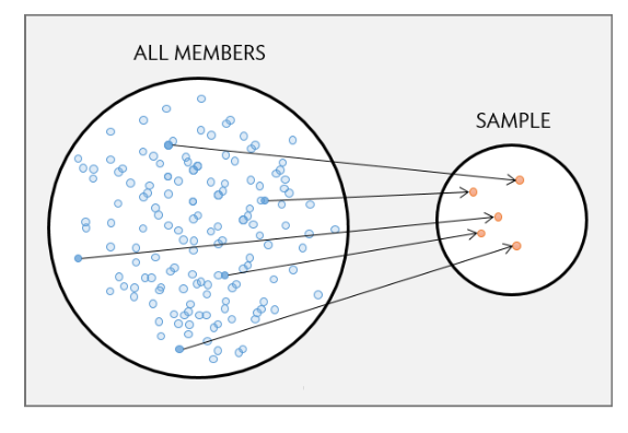
Sampling establishes the link (or lack thereof) between a sample and a population.

In a simple random sample, units are chosen in such a way that every individual in the population has an equal probability of inclusion. For the SRS:
- sample statistics mirror population statistics (sample is representative)
- sampling variability depends only on population variability and sample size
Population models
Inference consists in using statistics of a random sample to ascertain population statistics under a population model.
A population model represents the distribution of values you’d see if you measured every individual in the study population. We think of the sample values as a random draw.


(Density is an alternative scale to frequency that is independent of population size.)
Point estimates
Sample statistics, viewed as guesses for the values of population statistics, are called ‘point estimates’.
We’ll focus on inferences involving the following:
| Population statistic | Parameter | Point estimate |
|---|---|---|
| Mean | \(\mu\) | \(\bar{x}\) |
| Standard deviation | \(\sigma\) | \(s_x\) |
A difficulty
Different samples yield different estimates.

Sample means:
| sample.1 | sample.2 |
|---|---|
| 5.093 | 5.136 |
- estimates are close but not identical
- the population mean can’t be both 5.093 and 5.136
- probably neither estimate is exactly correct
Estimation error and sample-to-sample variability are inherent to point estimation.
Simulating sampling variability

These are 20 random samples with the sample mean indicated by the dashed line and the population distribution and mean overlaid in red.
- sample size \(n = 20\)
- frequency distributions differ a lot
- sample means differ some
We can actually measure this variability!
Simulating sampling variability
If we had means calculated from a much larger number of samples, we could make a frequency distribution for the values of the sample mean.

| sample | 1 | 2 | \(\cdots\) | 10,000 |
| mean | 4.957 | 5.039 | \(\cdots\) | 5.24 |
We could then use the usual measures of center and spread to characterize the distribution of sample means.
- mean of \(\bar{x}\): 5.0373228
- standard deviation of \(\bar{x}\): 0.2387869
Across 10,000 random samples of size 20, the typical sample mean was 5.04 and the root average squared distance of the sample mean from its typical value was 0.239.
Sampling distributions
What we are simulating is known as a sampling distribution: the frequency of values of a statistic across all possible random samples.

Provided data are from a random sample, the sample mean \(\bar{x}\) has a sampling distribution with
- mean \(\color{red}{\mu}\) (population mean)
- standard deviation \(\color{red}{\frac{\sigma}{\sqrt{n}}}\)
regardless of its exact form.
In other words, across all random samples of a fixed size…
- The average value of the sample mean is the population mean.
- The average squared error (sample mean - population mean)\(^2\) is \(\frac{\sigma^2}{n}\)
Effect of sample size
The standard deviation of the sampling distribution of \(\bar{x}\) is inversely proportional to sample size.

As sample size increases…
- accuracy remains the same
- estimates get more precise
- skewness vanishes
Measuring sampling variability
In practice \(\sigma\) is not known so we use an estimate of sampling variability known as a standard error: \[ SE(\bar{x}) = \frac{s_x}{\sqrt{n}} \qquad \left(\frac{\text{sample SD}}{\sqrt{\text{sample size}}}\right) \]
For example:

\[ SE(\bar{x}) = \frac{1.073}{\sqrt{20}} = 0.240 \]
The root average squared error of the sample mean is estimated to be 0.240 mmol/L.
Reporting point estimates
It is common style to report the value of a point estimate with a standard error given parenthetically.
Statistics from full NHANES sample:
| mean | sd | n |
|---|---|---|
| 5.043 | 1.075 | 3179 |
The mean total cholesterol among the population is estimated to be 5.043 mmol/L (SE 0.019)
This style of report communicates:
- parameter of interest
- value of point estimate
- error/variability of point estimate
Interval estimation
An interval estimate is a range of plausible values for a population parameter.
The general form of an interval estimate is: \[\text{point estimate} \pm \text{margin of error}\]
A common interval for the population mean is: \[\bar{x} \pm 2\times SE(\bar{x}) \qquad\text{where}\quad SE(\bar{x}) = \left(\frac{s_x}{\sqrt{n}}\right)\]
By hand: \[5.043 \pm 2\times 0.0191 = (5.005, 5.081)\]

STAT218