2.79, 2.93, 3.22, 3.78, 3.22, 3.38, 3.18, 3.33, 3.34, 3.06, 3.07, 3.56, 3.08, 4.64 and 3.34
Two sample inference
Hypothesis tests and intervals for comparing two population means
Today’s agenda
- [lecture] two sample inference; statistical power
- [lab] two-sample \(t\) tests in R
Two-sample inference
Review: one-sample inference
The following are 15 measurements of the pesticide DDT in kale in parts per million (ppm).
C. E. Finsterwalder (1976) Collaborative study of an extension of the Mills et al method for the determination of pesticide residues in food. J. Off. Anal. Chem. 59, 169–171.
Imagine the target level for safety considerations is 3ppm or less, and you want to use this data to determine whether the mean DDT level is within safe limits.
\[ \begin{cases} H_0: &\mu = 3 \quad(\text{null hypothesis})\\ H_A: &\mu > 3 \quad(\text{alternative hypothesis}) \end{cases} \]
We choose this direction because we’re concerned with evidence that mean DDT exceeds the threshold.
Review: one-sample inference
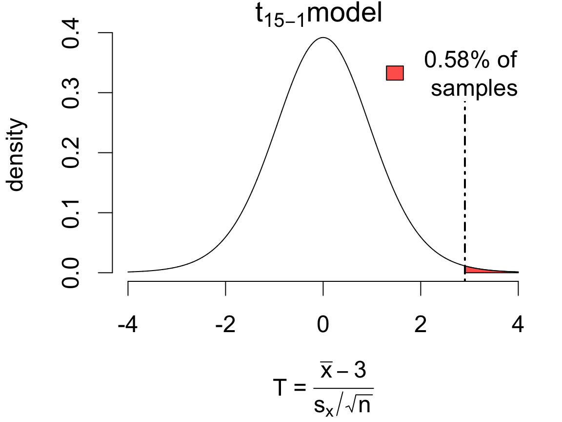
If in fact \(\mu = 3\), then according to the \(t\) model 0.58% of samples would produce an error of this magnitude or more in the direction of the alternative:
    One Sample t-test

data:  ddt
t = 2.9059, df = 14, p-value = 0.005753
alternative hypothesis: true mean is greater than 3
95 percent confidence interval:
 3.129197      Inf
sample estimates:
mean of x
    3.328
The data provide strong evidence that mean DDT in kale exceeds 3ppm (T = 2.9059 on 14 degrees of freedom, p = 0.0058). With 95% confidence, the mean DDT is estimated to be at least 3.129, with a point estimate of 3.32 (SE: 0.1168).
Notice the one-sided interval! (Inf = \(\infty\).) This is called a “lower confidence bound”.
Testing a mean difference
Does the average U.S. adult wish to lose weight?
| subject | actual | desired | difference |
|---|---|---|---|
| 1 | 265 | 225 | 40 |
| 2 | 150 | 150 | 0 |
| 3 | 137 | 150 | -13 |
| 4 | 159 | 125 | 34 |
| 5 | 145 | 125 | 20 |
    One Sample t-test

data:  weight.diffs
t = 4.2172, df = 59, p-value = 4.311e-05
alternative hypothesis: true mean is greater than 0
95 percent confidence interval:
 10.99824      Inf
sample estimates:
mean of x
 18.21667
The data provide evidence that the average U.S. adult’s actual weight exceeds their desired weight (T = 4.2172 on 59 degrees of freedom, p < 0.0001).
Inference here is on the mean difference: \(H_0: \delta = 0\) vs. \(H_A: \delta > 0\).
Can we also do inference on a difference in means?
Testing a difference in means
Peter and Rosemary Grant caught and measured birds from more than 20 generations of finches on Daphne Major.
severe drought in 1977 limited food to large tough seeds
selection pressure favoring larger and stronger beaks
hypothesis: beak depth increased in 1978 relative to 1976
| year | depth |
|---|---|
| 1976 | 10.8 |
| 1976 | 7.4 |
| 1978 | 11.4 |
| 1978 | 10.6 |
To answer this, we need to test a hypothesis involving two means:
\[ \begin{cases} H_0: &\mu_{1976} = \mu_{1978} \\ H_A: &\mu_{1976} < \mu_{1978} \end{cases} \]
- can’t do inference on a mean difference here (no pairing of observations)
- treat each year as an independent sample
Two-sample \(t\)-test
If \(x_1, \dots, x_{58}\) are the 1976 observations and \(y_1, \dots, y_{65}\) are the 1978 observations:
- \(\bar{x}\) is a point estimate for \(\mu_{1976}\) with standard error \(SE(\bar{x}) = \frac{s_x}{\sqrt{n_x}}\)
- \(\bar{y}\) is a point estimate for \(\mu_{1978}\) with standard error \(SE(\bar{y}) = \frac{s_y}{\sqrt{n_y}}\)
Inference uses a new \(T\) statistic:
\[ T = \frac{(\bar{x} - \bar{y}) - \delta_0}{SE(\bar{x} - \bar{y})} \]
- \(\delta_0\) is the hypothesized difference in means
- \(SE(\bar{x} - \bar{y}) = \sqrt{SE(\bar{x})^2 + SE(\bar{y})^2}\)
- \(t_\nu\) model approximates the sampling distribution when each sample meets assumptions for one-sample inference
Performing the test (by hand)
| year | depth.mean | depth.sd | n |
|---|---|---|---|
| 1976 | 9.453 | 0.9625 | 58 |
| 1978 | 10.19 | 0.8073 | 65 |
Point estimates: \[ \begin{align*} \bar{x} &= \qquad\qquad\qquad\qquad\\ \bar{y} &= \\ SE(\bar{x}) &= \\ SE(\bar{y}) &= \end{align*} \] Hypotheses: \[ \begin{cases} H_0: &\mu_{1976} - \mu_{1978} = 0 \\ H_A: &\mu_{1976} - \mu_{1978} < 0 \end{cases} \]
Test statistic: \[ \begin{align*} \bar{x} - \bar{y} &= \qquad\qquad\qquad\qquad\qquad\qquad\\ SE(\bar{x} - \bar{y}) &= \sqrt{SE(\bar{x})^2 + SE(\bar{y})^2} = \\ T &= \frac{(\bar{x} - \bar{y}) - \delta_0}{SE(\bar{x} - \bar{y})} = \end{align*} \] Conclusion: [reject]/[fail to reject] \(H_0\) in favor of \(H_A\)
How can you tell without the exact \(p\) value?
Performing the test (in R)
Welch Two Sample t-test
data: depth by year
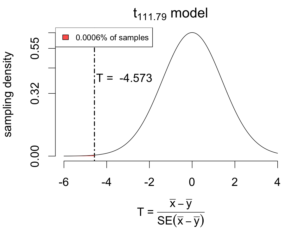
t = -4.5727, df = 111.79, p-value = 6.255e-06
alternative hypothesis: true difference in means between group 1976 and group 1978 is less than 0
95 percent confidence interval:
-Inf -0.4698812
sample estimates:
mean in group 1976 mean in group 1978
9.453448 10.190769 The data provide evidence that mean beak depth increased following the drought (T = -4.5727 on 111.79 degrees of freedom, p < 0.0001). With 95% confidence, the mean increase is estimated to be at least 0.4699 mm, with a point estimate of 0.7373 (SE 0.1612).
Highly similar to the one-sample \(t\)-test, but notice:
- input is a formula
depth ~ year(“depth depends on year”) and data framefinch munow indicates hypothesized difference in means \(\delta_0\)- decimal degrees of freedom
- alternative is relative to the order in which groups appear
Checking test assumptions
The two-sample test is appropriate whenever two one-sample tests would be.
In other words, the test assumes that both samples are either:
- sufficiently large; or
- have little skew and few outliers
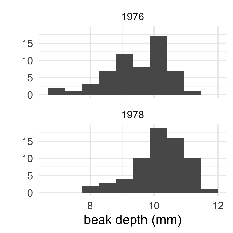
To check, simply inspect each histogram.
- both distributions unimodal
- both a bit left skewed
- no extreme outliers
- large sample sizes (58, 65)
Checking test assumptions
The two-sample test is appropriate whenever two one-sample tests would be.
In other words, the test assumes that both samples are either:
- sufficiently large; or
- have little skew and few outliers
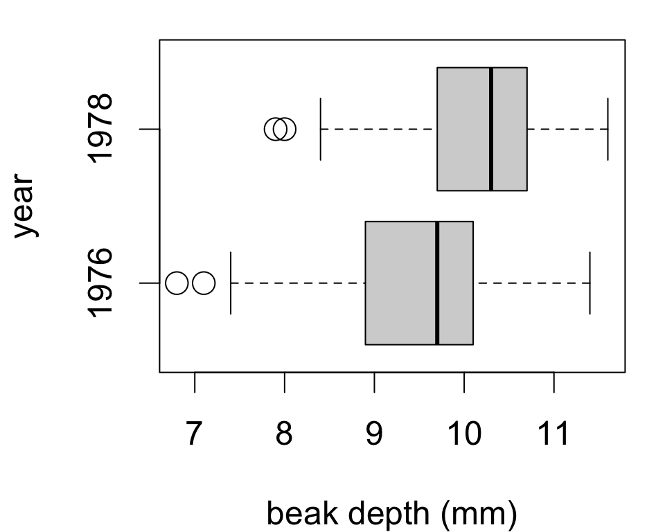
Could also check side-by-side boxplots for:
- approximate symmetry of boxes
- outliers far from whiskers
This is also a nice visualization of differences between samples.
Cloud data
Does seeding clouds with silver iodide increase mean rainfall?
Data are rainfall measurements in a target area from 26 days when clouds were seeded and 26 days when clouds were not seeded.
rainfallgives volume of rainfall in acre-feettreatmentindicates whether clouds were seeded
Hypotheses to test: \[ \begin{cases} H_0: &\mu_\text{seeded} = \mu_\text{unseeded} \\ H_A: &\mu_\text{seeded} > \mu_\text{unseeded} \end{cases} \]
| rainfall | treatment |
|---|---|
| 334.1 | seeded |
| 489.1 | seeded |
| 200.7 | seeded |
| 40.6 | seeded |
| 21.7 | unseeded |
| 17.3 | unseeded |
| 68.5 | unseeded |
| 830.1 | unseeded |
Cloud data: which test?
Does seeding clouds with silver iodide increase mean rainfall?
    Welch Two Sample t-test

data:  rainfall by treatment
t = 1.9982, df = 33.855, p-value = 0.9731
alternative hypothesis: true difference in means between group seeded and group unseeded is less than 0
95 percent confidence interval:
     -Inf 512.1582
sample estimates:
  mean in group seeded mean in group unseeded
              441.9846               164.5885
    Welch Two Sample t-test

data:  rainfall by treatment
t = 1.9982, df = 33.855, p-value = 0.02689
alternative hypothesis: true difference in means between group seeded and group unseeded is greater than 0
95 percent confidence interval:
 42.63408      Inf
sample estimates:
  mean in group seeded mean in group unseeded
              441.9846               164.5885
You can tell which group R considers first based on which estimate is printed first.
'greater'is interpreted as [FIRST GROUP] > [SECOND GROUP]'less'is interpreted as [FIRST GROUP] < [SECOND GROUP]
Cloud data: interpretation
Does seeding clouds with silver iodide increase mean rainfall?
    Welch Two Sample t-test

data:  rainfall by treatment
t = 1.9982, df = 33.855, p-value = 0.02689
alternative hypothesis: true difference in means between group seeded and group unseeded is greater than 0
95 percent confidence interval:
 42.63408      Inf
sample estimates:
  mean in group seeded mean in group unseeded
              441.9846               164.5885
The data provide evidence that cloud seeding increases mean rainfall (T = 1.9982 on 33.855 degrees of freedom, p = 0.02689). With 95% confidence, seeding is estimated to increase mean rainfall by at least 42.63 acre-feet, with a point estimate of 277.4 (SE 138.8199).
Statistical power
\(p\)-values and type I errors
A \(p\)-value captures how often you’d make a mistake if \(H_0\) were true.
    Welch Two Sample t-test

data:  rainfall by treatment
t = 1.9982, df = 33.855, p-value = 0.02689
alternative hypothesis: true difference in means between group seeded and group unseeded is greater than 0
95 percent confidence interval:
 42.63408      Inf
sample estimates:
  mean in group seeded mean in group unseeded
              441.9846               164.5885
If there is no effect of cloud seeding, then we would see \(T > 1.9982\) for 2.69% of samples.
While unlikely, our sample could have been among that 2.69%
By rejecting here we are willing to be wrong 2.69% of the time
Type II errors
But you can also make a mistake when \(H_0\) is false!
    Welch Two Sample t-test

data:  rainfall by treatment
t = 1.9982, df = 33.855, p-value = 0.02689
alternative hypothesis: true difference in means between group seeded and group unseeded is greater than 0
95 percent confidence interval:
 42.63408      Inf
sample estimates:
  mean in group seeded mean in group unseeded
              441.9846               164.5885
Suppose we test at the 1% level.
The test fails to reject (\(p > 0.01\)), but that doesn’t completely rule out \(H_A\).
The estimated effect – an increase of 277.4 acre-feet – could be too small relative to the variability in rainfall.
Simulating type II errors
Summary stats for cloud data:
| treatment | mean | sd | n |
|---|---|---|---|
| seeded | 442 | 650.8 | 26 |
| unseeded | 164.6 | 278.4 | 26 |
We can approximate the type II error rate by:
- simulating datasets with matching statistics
- performing upper-sided tests of no difference
- computing the proportion of fail-to-reject decisions

If in fact the effect size is exactly 277, a level 1% test with similar data will fail to reject 80.3% of the time!
Larger effect size
Summary stats for cloud data:
| treatment | mean | sd | n |
|---|---|---|---|
| seeded | 442 | 650.8 | 26 |
| unseeded | 164.6 | 278.4 | 26 |
Type II error rate depends on effect size:
- larger effect \(\longrightarrow\) lower error rate

If in fact the effect size is exactly 400, a level 1% test with similar data will fail to reject 57.9% of the time.
Smaller effect size
Summary stats for cloud data:
| treatment | mean | sd | n |
|---|---|---|---|
| seeded | 442 | 650.8 | 26 |
| unseeded | 164.6 | 278.4 | 26 |
Type II error rate depends on effect size:
- larger effect \(\longrightarrow\) lower error rate
- smaller effect \(\longrightarrow\) higher error rate

If in fact the effect size is exactly 100, a level 1% test with similar data will fail to reject 96.3% of the time.
Statistical power
The power of a test refers to its true rejection rate under an alternative and is defined as: \[\beta = \underbrace{(1 - \text{type II error rate})}_\text{correct decision rate when null is false}\]
Power is often interpreted as a detection rate:
- high type II error \(\longrightarrow\) low power \(\longrightarrow\) low detection rate
- low type II error \(\longrightarrow\) high power \(\longrightarrow\) high detection rate
Power depends on the exact alternative scenario:
- low for alternatives close to the null value
- high for alternatives far from the null value
(Here “close” and “far” is relative to sampling variability.)
Power curves
Power is usually represented as a curve depending on the true difference.
Power curve for the test applied to the cloud data:

Assumptions:
- sample size \(n = 26\)
- significance level \(\alpha = 0.05\)
- population standard deviation \(\sigma = 650\) (larger of two group estimates)
Post-hoc power analysis
Can we estimate the power of a test we already performed?
Feasible if we assume (a) a population standard deviation and (b) test conditions are met.
For the cloud seeding test:
power.t.test(delta = 250, # magnitude of difference
             sd = 650, # largest population SD
             n = 26, # smallest sample size
             sig.level = 0.01,
             type = 'two.sample',
             alternative = 'one.sided')
     Two-sample t test power calculation

              n = 26
          delta = 250
             sd = 650
      sig.level = 0.01
          power = 0.1643217
    alternative = one.sided

NOTE: n is number in *each* group
For a conservative estimate, use:
- smallest of the two sample sizes
- largest of the two standard deviations
- smaller difference than observed
\(\Longrightarrow\) our test would only reject in favor of a difference of the observed magnitude about 16% of the time
Failure to reject doesn’t strongly rule out the alternative.
Sample size calculation
If you were (re)designing the study, how much data should you collect to detect a specified effect size?
To detect a difference of 250 or more due to cloud seeding with power 0.9:
power.t.test(power = 0.9, # target power level
             delta = 250, # smallest difference
             sd = 650, # largest population SD
             sig.level = 0.01,
             type = 'two.sample',
             alternative = 'one.sided')
     Two-sample t test power calculation

              n = 177.349
          delta = 250
             sd = 650
      sig.level = 0.01
          power = 0.9
    alternative = one.sided

NOTE: n is number in *each* group
For a conservative estimate, use:
- overestimate of the larger of the two standard deviations
- minimum difference of interest
\(\Longrightarrow\) we need at least 177 observations in each group to detect a difference of 250 or more at least 90% of the time
Practical constraints
Minimum detectable difference at 5 levels of power as a function of sample size for a one-sided test:

Assumes \(\sigma = 650\) for a conservative estimate.
Pilots and planes are expensive, so \(n = 177\) may be infeasible.
Some alternatives:
decrease target power \(\beta\)
- \(\beta = 0.6, \delta=250, \alpha = 0.01\) \(\longrightarrow\) \(n =92\)
increase target difference \(\delta\)
- \(\beta = 0.6, \delta=350, \alpha = 0.01\) \(\longrightarrow\) \(n =48\)
increase test level \(\alpha\)
- \(\beta = 0.6, \delta=350, \alpha = 0.05\) \(\longrightarrow\) \(n =26\)
Revisiting body temperatures
Does mean body temperature differ between men and women?

Test \(H_0: \mu_F = \mu_M\) against \(H_A: \mu_F \neq \mu_M\)
    Welch Two Sample t-test

data:  body.temp by sex
t = 1.7118, df = 34.329, p-value = 0.09595
alternative hypothesis: true difference in means between group female and group male is not equal to 0
95 percent confidence interval:
 -0.09204497  1.07783444
sample estimates:
mean in group female   mean in group male
            98.65789             98.16500
Suggestive but insufficient evidence that mean body temperature differs by sex.
Notice: estimated difference (F - M) is 0.493 °F (SE 0.2879)
What if we had more data?
Here are estimates from two larger samples of 65 individuals each (compared with 19, 20):
| sex | mean.temp | se | n |
|---|---|---|---|
| female | 98.39 | 0.09222 | 65 |
| male | 98.1 | 0.08667 | 65 |
- estimated difference (F - M) is smaller 0.2892 °F
- but so is the standard error SE 0.1266 (recall more data \(\longleftrightarrow\) better precision)
    Welch Two Sample t-test

data:  body.temp by sex
t = 2.2854, df = 127.51, p-value = 0.02394
alternative hypothesis: true difference in means between group female and group male is not equal to 0
95 percent confidence interval:
 0.03881298 0.53964856
sample estimates:
mean in group female   mean in group male
            98.39385             98.10462
The data provide evidence that mean body temperature differs by sex (T = 2.29 on 127.51 degrees of freedom, p = 0.02394).
Power calculations
| sex | btemp.mean | btemp.sd | n |
|---|---|---|---|
| female | 98.39 | 0.7435 | 65 |
| male | 98.1 | 0.6988 | 65 |
Estimated difference: 0.29 °F.
In this case, a 5% level test will detect a 0.25-degree difference over 90% of the time when \(n = 200\).
A statistical trap
If you collect enough data, you can detect an arbitrarily small difference in means almost always.

So keep in mind:
- statistical significance \(\neq\) practical significance
- large samples will tend to produce statistically significant results
It’s a good idea to always check your point estimates and ask whether findings are practically meaningful.
Extras
The equal-variance \(t\)-test
If it is reasonable to assume the (population) standard deviations are the same in each group, one can gain a bit of power by using a different standard error:
\[SE_\text{pooled}(\bar{x} - \bar{y}) = \sqrt{\frac{\color{red}{s_p^2}}{n_x} + \frac{\color{red}{s_p^2}}{n_y}} \quad\text{where}\quad \color{red}{s_p} = \underbrace{\sqrt{\frac{(n_x - 1)s_x^2 + (n_y - 1)s_y^2}{n_x + n_y - 2}}}_{\text{weighted average of } s_x^2 \;\&\; s_y^2}\]
Implement by adding var.equal = T as an argument to t.test().
- larger df is used, hence more frequent rejections
- avoid unless you have a small sample
STAT218
Two sample inference Hypothesis tests and intervals for comparing two population means