Post-hoc inference in ANOVA
Contrasts between group means
Today’s agenda
- [lecture] post-hoc inference for contrasts in ANOVA
- [lab] estimates, tests, and intervals using
emmeans
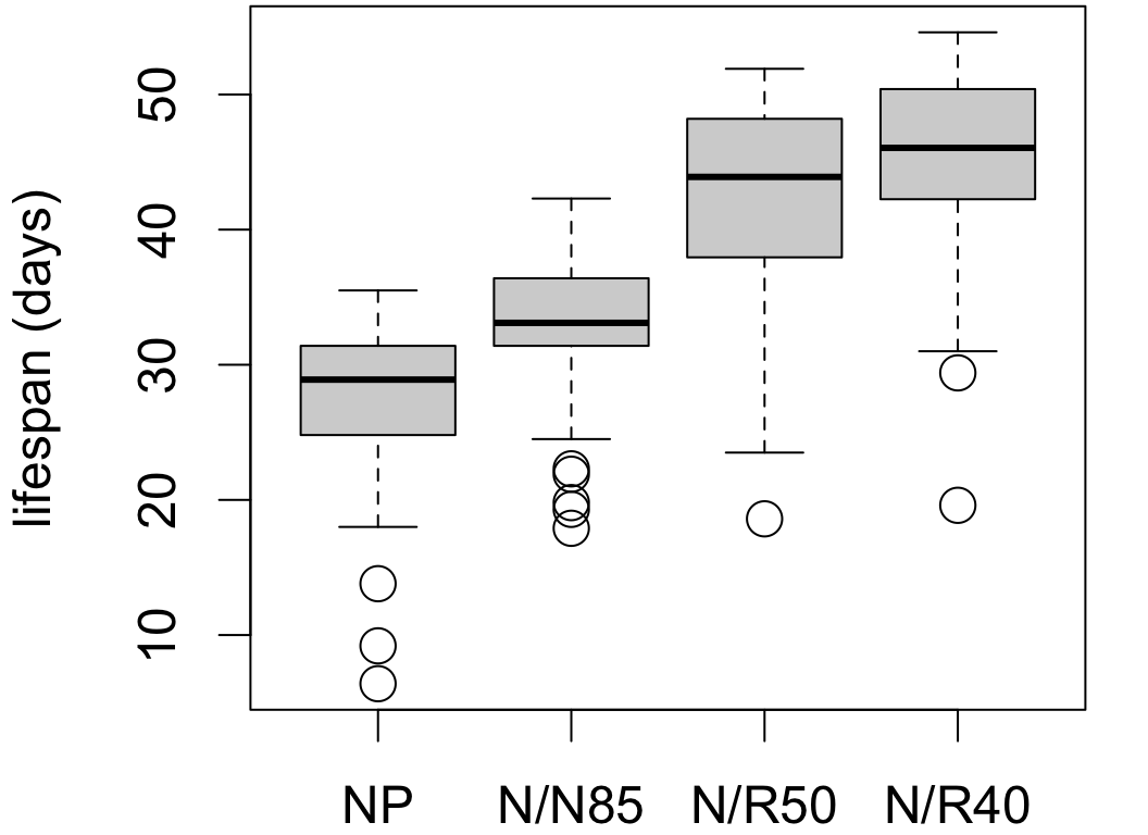
Diet restriction and longevity
H0:μNP=μN/N85=μN/R50=μN/R40HA:at least two means differ
             Df Sum Sq Mean Sq F value Pr(>F)
diet          3  11426    3809   87.41 <2e-16 ***
Residuals   233  10152      44
---
Signif. codes: 0 '***' 0.001 '**' 0.01 '*' 0.05 '.' 0.1 ' ' 1# Effect Size for ANOVA (Type I)
Parameter | Eta2 | 95% CI
-------------------------------
diet | 0.53 | [0.44, 0.60]The data provide evidence that caloric restriction affects mean lifespan (F = 87.41 on 3 and 233 degrees of freedom, p < 0.0001). With 95% confidence, an estimated 44%-60% of variability in lifespans is attributable to caloric intake.
Post-hoc inference in ANOVA
The ANOVA tells us there’s evidence that caloric intake affects mean lifespan. So now that we’ve inferred an effect, we might want to know:
- What are the mean lifespans for each level of restriction?
- Which means differ?
- How do restricted-calorie diets compare with the control (NP)?
We can answer these questions with post-hoc (after-the-fact) inferences on:
- group means μi
- “contrasts” μi−μj
Estimates for group means
Interval estimates for group means in ANOVA are similar to marginal confidence intervals except for two details.
| diet | estimate | SE | 95% CI |
|---|---|---|---|
| NP | 27.4 | 0.943 | (25.54, 29.26) |
| N/N85 | 32.69 | 0.8743 | (30.97, 34.41) |
| N/R50 | 42.3 | 0.7834 | (40.75, 43.84) |
| N/R40 | 45.12 | 0.8522 | (43.44, 46.8) |
- Standard errors are based on a “pooled” standard deviation:
SEi=spooled√ni=√MSE√ni
- Critical values are from a tn−k model (instead of tn−1).
Rationale:
- the ANOVA model assumes equal variability (standard deviations) across groups
- better precision (for variability estimates, not means) when assumption holds
Simultaneous intervals
For multiple intervals we can distinguish two types of coverage.
- individual coverage: how often one interval covers the population mean
- simultaneous coverage: how often all intervals cover population means at the same time

The Bonferroni correction for k intervals consists in changing the individual coverage level to (1−αk)%.
- Effectively a width increase
- Guarantees joint coverage (1−α)%
- Tends to be over conservative with many means (large k)
Implementation in R
 diet  emmean    SE  df lower.CL upper.CL
 NP      27.4 0.943 233     25.0     29.8
 N/N85   32.7 0.874 233     30.5     34.9
 N/R50   42.3 0.783 233     40.3     44.3
 N/R40   45.1 0.852 233     43.0     47.3

Confidence level used: 0.95
Conf-level adjustment: bonferroni method for 4 estimates - note Bonferroni adjustment
- these are model-based estimates that depend on the fitted ANOVA model

Caution: these intervals do NOT indicate which means differ significantly.
Pairwise comparisons
The difference μNP−μN/N85 is an example of a “contrast” involving two means.
Simultaneous inference on pairwise contrasts will determine which means differ and by how much.
| difference | estimate | SE |
|---|---|---|
| NP - (N/N85) | -5.289 | 1.286 |
| NP - (N/R50) | -14.9 | 1.226 |
| NP - (N/R40) | -17.71 | 1.271 |
| (N/N85) - (N/R50) | -9.606 | 1.174 |
| (N/N85) - (N/R40) | -12.43 | 1.221 |
| (N/R50) - (N/R40) | -2.819 | 1.158 |
Remarks:
point estimates are ˉxi−ˉxj
SEij=SE(ˉxi−ˉxj)=spooled√1ni+1nj
inference is based on a tn−k model
- degrees of freedom: n−k
- tests: Tij=ˉxi−ˉxjSEij
- intervals: ˉxi−ˉxj±c×SEij
Multiplicity corrections must adjust for the number of contrasts (6), not means (4).
Pairwise comparisons: tests
Which means differ significantly?
emmeans then contrast then test:
contrast estimate SE df t.ratio p.value
NP - (N/N85) -5.29 1.29 233 -4.113 0.0003
NP - (N/R50) -14.90 1.23 233 -12.150 <.0001
NP - (N/R40) -17.71 1.27 233 -13.938 <.0001
(N/N85) - (N/R50) -9.61 1.17 233 -8.183 <.0001
(N/N85) - (N/R40) -12.43 1.22 233 -10.177 <.0001
(N/R50) - (N/R40) -2.82 1.16 233 -2.436 0.0937
P value adjustment: bonferroni method for 6 tests - p-values are adjusted for multiplicity
- reject if adjusted p-value is below the significance threshold
Hypotheses for pairwise tests:
{H0:μi−μj=0HA:μi−μj≠0 Test statistic:
Tij=ˉxi−ˉxjSEij
p-values are obtained from a tn−k model for the sampling distribution of Tij.
Pairwise comparisons: tests
Which means differ significantly?
emmeans then contrast then test:
contrast estimate SE df t.ratio p.value
NP - (N/N85) -5.29 1.29 233 -4.113 0.0003
NP - (N/R50) -14.90 1.23 233 -12.150 <.0001
NP - (N/R40) -17.71 1.27 233 -13.938 <.0001
(N/N85) - (N/R50) -9.61 1.17 233 -8.183 <.0001
(N/N85) - (N/R40) -12.43 1.22 233 -10.177 <.0001
(N/R50) - (N/R40) -2.82 1.16 233 -2.436 0.0937
P value adjustment: bonferroni method for 6 tests The data provide evidence at the 5% significance level that mean lifespan differs among all levels of diet restriction except the N/R40 and N/R50 groups (p = 0.0937), for which the evidence is suggestive but inconclusive.
Multiple testing correction matters
Using unadjusted p-values will inflate type I error rates.
setting adjust = 'none':
contrast estimate SE df t.ratio p.value
NP - (N/N85) -5.29 1.29 233 -4.113 0.0001
NP - (N/R50) -14.90 1.23 233 -12.150 <.0001
NP - (N/R40) -17.71 1.27 233 -13.938 <.0001
(N/N85) - (N/R50) -9.61 1.17 233 -8.183 <.0001
(N/N85) - (N/R40) -12.43 1.22 233 -10.177 <.0001
(N/R50) - (N/R40) -2.82 1.16 233 -2.436 0.0156Failure to adjust for multiple inferences leads to a different conclusion:
The data provide evidence at the 5% significance levelthat mean lifespan differs among all levels of diet restriction.
This is incorrect, because the joint significance level is not 5%.
Without adjustment, type I error could be as high as k×α=6×0.05=0.3.
Pairwise comparisons: intervals
How much do means differ?
emmeans then contrast then confint:
emmeans(object = fit, specs = ~ diet) |>
contrast('pairwise') |>
confint(level = 0.95, adjust = 'bonferroni') contrast estimate SE df lower.CL upper.CL
NP - (N/N85) -5.29 1.29 233 -8.71 -1.867
NP - (N/R50) -14.90 1.23 233 -18.16 -11.633
NP - (N/R40) -17.71 1.27 233 -21.10 -14.333
(N/N85) - (N/R50) -9.61 1.17 233 -12.73 -6.482
(N/N85) - (N/R40) -12.43 1.22 233 -15.67 -9.177
(N/R50) - (N/R40) -2.82 1.16 233 -5.90 0.261
Confidence level used: 0.95
Conf-level adjustment: bonferroni method for 6 estimates levelspecifies joint coverage after adjustment
Intervals are for the contrast μi−μj:
ˉxi−ˉxj±c×SEij
The critical value c is obtained from the tn−k model.
For a (1−α)×100% confidence interval with Bonferroni correction:
c=(1−α2k)quantile
Pairwise comparisons: intervals
How much do means differ?
emmeans then contrast then confint:
emmeans(object = fit, specs = ~ diet) |>
  contrast('pairwise') |>
  confint(level = 0.95, adjust = 'bonferroni')
contrast estimate SE df lower.CL upper.CL
NP - (N/N85) -5.29 1.29 233 -8.71 -1.867
NP - (N/R50) -14.90 1.23 233 -18.16 -11.633
NP - (N/R40) -17.71 1.27 233 -21.10 -14.333
(N/N85) - (N/R50) -9.61 1.17 233 -12.73 -6.482
(N/N85) - (N/R40) -12.43 1.22 233 -15.67 -9.177
(N/R50) - (N/R40) -2.82 1.16 233 -5.90 0.261
Confidence level used: 0.95
Conf-level adjustment: bonferroni method for 6 estimates Interpretations are the same as usual:
With 95% confidence, mean lifespan on a normal diet is estimated to exceed mean lifespan on an unrestricted diet by between 1.87 and 8.71 days, with a point estimate of 5.29 days difference (SE 1.29).
Pairwise comparisons: visualizations
Another option is to visualize the pairwise comparison inferences by displaying simultaneous 95% intervals.
Easy to spot significant contrasts:
- intervals exclude 0 ⇔ tests reject

Comparisons with a control
Does diet restriction increase mean lifespan, and if so by how much?
Specify contrast('trt.vs.ctrl'):
| contrast | estimate | SE | 95% CI |
|---|---|---|---|
| (N/N85) - NP | 5.289 | 1.286 | (2.23, 8.34) |
| (N/R50) - NP | 14.9 | 1.226 | (11.98, 17.81) |
| (N/R40) - NP | 17.71 | 1.271 | (14.7, 20.73) |
Multiple inference adjustment uses Dunnett’s method
- specialized correction for comparisons with a control
adjust = 'dunnett'
Comparisons will be relative to first group or factor level in R
With 95% confidence, relative to an unrestricted diet…
- a 85kcal/day diet increases lifespan by an estimated 2.23 to 8.34 days
- a 50kcal/day diet increases lifespan by an estimated 11.98 to 17.81 days
- a 40kcal/day diet increases lifespan by an estimated 14.70 to 20.73 days
Extras
Log contrasts: relative change
Can we instead estimate a percent change in lifespan relative to the control?
The contrast in log-lifetimes would be:
log(μN85)−log(μNP)=log(μN85μNP) So to answer the question:
- refit the ANOVA model with log lifetimes
- compute contrasts with control group using Dunnett’s method
- exponentiate estimates to obtain ratios (and hence percentages)
| contrast | estimate | 95% CI |
|---|---|---|
| (N/R50)/NP | 1.572 | (1.42, 1.73) |
| (N/R40)/NP | 1.688 | (1.52, 1.87) |
Fact: mean log lifetime = log median lifetime.
With 95% confidence, diet restriction to 40kcal (a 52.9% reduction relative to an 85kCal diet) is estimated to increase median lifespan in mice by 52% to 87%.
Extra credit: work out and interpret the interval estimate for the contrast not shown above.
Response curve
We can use the log-contrasts to estimate a response curve relating caloric reduction and change in median lifespan.

Simplifying heuristics:
- percent increase in median lifespan (y axis) is relative to unrestricted (NP) diet
- percent reduction in caloric intake (x axis) is relative to 85kCal diet
STAT218
Post-hoc inference in ANOVA Contrasts between group means