STAT218 - Simple linear regression

Today’s agenda

[lab] Line fitting
[lecture] Least squares estimation

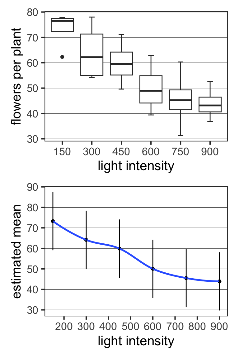
Meadowfoam flowering

Mean flowering depends on light intensity.

the “response” variable is flowers per plant
the “explanatory” variable is light intensity

In an ANOVA model, the explanatory variable is treated as categorical.

one mean estimated per unique value of the explanatory variable
values usually fixed in advance by researcher

What if light intensity instead varied continuously?

Could we estimate mean flowering as a continuous function of intensity?

PREVEND data

Ruff Figural Fluency Test (RFFT) is a cognitive assessment.

measures nonverbal fluency and executive cognitive function
scale: 0 (worst) to 175 (best)

casenr	age	rfft
126	37	136
33	36	80
145	37	102
146	37	85

Question of interest:

How much does cognitive ability as measured by RFFT decline with age on average?

PREVEND data

Ruff Figural Fluency Test (RFFT) is a cognitive assessment.

measures nonverbal fluency and executive cognitive function
scale: 0 (worst) to 175 (best)

casenr	age	rfft
126	37	136
33	36	80
145	37	102
146	37	85

A straight line seems to describe the RFFT-age relationship well enough.

This suggests a model:

mean RFFT is a linear function of age
remaining variation in RFFT is random

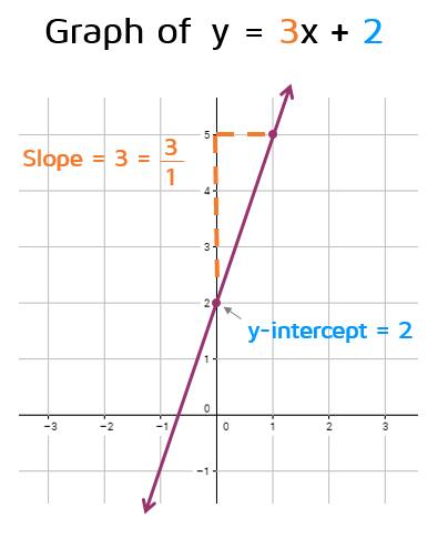
Lines

The equation of a line in slope-intercept form is:

$y = a x + b$

$a$ is the slope (rise over run) and $b$ is the intercept:

the line crosses the $y$ axis at $b$
$y$ changes by $a$ per unit increment in $x$

There is exactly one line through any two points.

Linear trends in data

We say a set of data points $(x_{i}, y_{i})$ exhibit a linear trend if the points fall “near” a line.

Some things to keep in mind:

real data will never fall exactly on a line
there may be outliers (e.g., red point at right)
points could be pretty far spread out and still exhibit a linear trend

Linear trends in data

We can articulate two properties of linear trends:

direction: positive (A) or negative (B)
strength: concentration about line

Note that trends in each row are identical.

Correlation

Correlation is a signed measure of strength of linear relationship.

$r = \frac{\sum_{i} (x_{i} - \bar{x}) (y_{i} - \bar{y})}{s_{x} \times s_{y}}$

When data points are far from the mean at the same time in the same direction, the magnitude will be larger.

sign indicates direction of relationship
magnitude indicates strength (always between -1 and 1)

Common mistake: strength $\neq$ slope.

Line fitting activity

Correlation between age and RFFT:

cor(age, rfft)

[1] -0.635854

negative relationship (sign)
moderate strength

But how do we find a line that describes the trend?

Best-fitting line

$RFFT = 134.098 - 1.191 \times age$

With each year of age, RFFT decreases by 1.191 points on average.

$\begin{aligned} slope : - 1.191 & = cor (age, RFFT) \times \frac{S D (RFFT)}{S D (age)} \\ intercept : 134.098 & = mean (RFFT) - (- 1.191) \times mean (age) \end{aligned}$

Bias and error

Bias and error are measured via residuals: $e_{i} = y_{i} - {\hat{y}}_{i}$

$bias = - \frac{1}{n} \sum_{i} e_{i}$
$SSE = \sum_{i} {e_{i}}^{2}$

The best-fitting line achieves two conditions:

no bias: underestimates and overestimates equally often
minimal error: as close as possible to as many data points as possible

The SLR model

The simple linear regression model is:

$Y = \underset{mean}{\underset{⏟}{β_{0} + β_{1} x}} + \underset{error}{\underset{⏟}{ϵ}}$

continuous response $Y$
explanatory variable $x$
regression coefficients $β_{0}, β_{1}$
model error $ϵ$

The values that minimize error subject to the model being unbiased are:

$\begin{aligned} {\hat{β}}_{0} & = \bar{y} - {\hat{β}}_{1} \bar{x} & (unbiased) \\ {\hat{β}}_{1} & = \frac{s_{y}}{s_{x}} \times r & (minimizes SSE) \end{aligned}$

These are called the least squares estimates.

Least squares estimates in R

According to the model, a one-unit increment in $x$ corresponds to a $β_{1}$ -unit change in mean $Y$ :

# fit model
fit <- lm(formula = rfft ~ age, data = prevend)
fit


Call:
lm(formula = rfft ~ age, data = prevend)

Coefficients:
(Intercept)          age  
    134.098       -1.191

With each additional year of age, mean RFFT score decreases by an estimated 1.191 points.

formula = <RESPONSE> ~ <EXPLANATORY> specifies the model
data = <DATAFRAME> specifies the observations

Error variability and model fit

The residual standard deviation provides an estimate of error variability:

$\hat{σ} = \sqrt{\frac{1}{n - 2} \sum_{i} e_{i}^{2}} (estimated error variability)$

The proportion of variability explained by the model is: $R^{2} = 1 - \frac{(n - 2) {\hat{σ}}^{2}}{(n - 1) s_{y}^{2}} (1 - \frac{error variability}{total variability})$

1 - (n - 2)*sigma(fit)^2/((n - 1)*var(rfft))

[1] 0.4043103

Age explains 40.43% of variability in RFFT.

Model specification

Is the relationship actually linear?

Two ways to check:

Inspect observed data for nonlinear trend
Inspect model residuals for “patterns”

Local smoothing is shown in blue.

The linear model is a fine approximation here – the curvature is very minor – but let’s consider an alternative model specification as a thought exercise.

An alternative model

$\log (RFFT) = β_{0} + β_{1} \times age + ϵ$

The model now implies that the mean RFFT score is a nonlinear function of age:

$RFFT \propto e^{β_{1} age}$

And we can still fit it using least squares:

lm(log(rfft) ~ age, data = prevend)


Call:
lm(formula = log(rfft) ~ age, data = prevend)

Coefficients:
(Intercept)          age  
    5.21739     -0.01951

Linear models can be used to capture more than just linear relationships!

Kleiber’s law

Kleiber’s law refers to the relationship between metabolic rate and body mass.

We can estimate it via the SLR model: $\log (metabolism) = β_{0} + β_{1} \log (mass) + ϵ$

Fitted model: $\log (metabolism) = 5.64 + 0.74 \times \log (mass)$

fit <- lm(log.metab ~ log.mass, data = kleiber)
fit


Call:
lm(formula = log.metab ~ log.mass, data = kleiber)

Coefficients:
(Intercept)     log.mass  
     5.6383       0.7387

Kleiber’s law: model interpretation

Exponentiating both sides of the fitted SLR model equation:

$\underset{e^{\log (metabolism)}}{\underset{⏟}{metabolism}} = \underset{e^{5.64}}{\underset{⏟}{280.99}} \times \underset{e^{0.74 \log (mass)}}{\underset{⏟}{{mass}^{0.74}}}$

So we’ve really estimated what’s known as a power law relationship: $y = a x^{b}$ .

multiplicative, not additive, relationship
doubling $x$ corresponds to changing $y$ by a factor of $2^{b}$

The estimate and interval for $β_{1}$ in the SLR model can be transformed appropriately for a more direct interpretation:

Every doubling of body mass is associated with an estimated 66.87% increase in median metabolism.