Inference for proportions
Today’s agenda
- [lecture] exact and approximate inference for one and two proportions
- [lab] tests for proportions in R
Categorical data
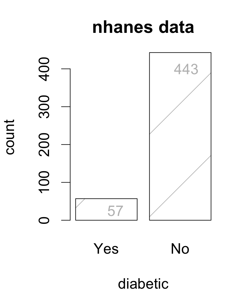
Consider the frequency of diabetes among a random sample of
- data values are Y/N
Can’t compute usual statistics (mean, variance, etc.), so…
- how should we summarize data?
- what population parameter(s) can we estimate?
- what statistical inferences are possible?
Sample proportions
Consider the sample proportion:
Interpreted as an estimate:
Diabetes prevalence among U.S. adults is estimated to be 11.4%.
So a natural parameter of interest is the true prevalence among all U.S. adults.
- in other words, the population proportion
But how to do inference?
Exact methods
Binomial probabilities
The chance that a randomly selected U.S. adult is diabetic is p.
The chance that two of three randomly selected U.S. adults are diabetic is:
The chance that x out of n randomly selected U.S. adults are diabetic is:

This is called a binomial probability distribution.
Exact sampling distribution
Suppose the true prevalence is 9.5%. Binomial probabilities give an exact sampling distribution for sample counts:

Inference methods for binary proportions based on the binomial are called exact because they use an exact sampling distribution rather than a model.
Upper-sided test
The data favor

    Exact binomial test

data:  57 and 500
number of successes = 57, number of trials = 500, p-value = 0.08745
alternative hypothesis: true probability of success is greater than 0.095
95 percent confidence interval:
 0.0913675 1.0000000
sample estimates:
probability of success
                 0.114
The data do not provide evidence that diabetes prevalence exceeds 9.5% (p = 0.0874).
Lower-sided test
The data favor

    Exact binomial test

data:  57 and 500
number of successes = 57, number of trials = 500, p-value = 0.9333
alternative hypothesis: true probability of success is less than 0.095
95 percent confidence interval:
 0.0000000 0.1401005
sample estimates:
probability of success
                 0.114
The data do not provide evidence that diabetes prevalence is less than 9.5% (p = 0.9333).
Two-sided test
The data favor

    Exact binomial test

data:  57 and 500
number of successes = 57, number of trials = 500, p-value = 0.1473
alternative hypothesis: true probability of success is not equal to 0.095
95 percent confidence interval:
 0.0874949 0.1451685
sample estimates:
probability of success
                 0.114
The data do not provide evidence that diabetes prevalence differs from 9.5% (p = 0.1473).
Exact confidence intervals
An exact confidence interval can be obtained by inverting the corresponding exact test.

With 90% confidence, diabetes prevalence among U.S. adults is estimated to be between 9.2% and 14%.
Unfortunately, this approach gives asymmetric intervals (midpoint is not
- choose smallest symmetric interval with exact coverage
- use a large-sample approximation
Approximate methods
SE for a sample proportion
Measure of spread for binomial data:
- highest when
- lowest when
Analogous to estimating a mean:

Sampling distribution of
The sample proportion
A common condition to check:

This model can be used to construct hypothesis tests and confidence intervals for
Confidence interval for
A confidence interval for a binomial proportion
The critical value
empirical rule:
for a
Confidence interval for
| p.hat | se | n |
|---|---|---|
| 0.114 | 0.01421 | 500 |
It is estimated that the proportion of the U.S. adult population with diagnosed diabetes is 11.4% (SE = 1.42%).
Check assumptions for the normal model:
95% confidence interval for diabetes prevalence:
With 95% confidence, the proportuion of U.S. adults with diagnosed diabetes is estimated to be between 8.81% and 14.59%.
Two-sided test
Test statistic:

The data provide no evidence that diabetes prevalence among U.S. adults differs from 9.5% (p = 0.1474).
(Another) Two-sided test
Test statistic:

The data provide evidence that diabetes prevalence among U.S. adults differs from 15% (p = 0.0242).
One-sided tests

The data provide no evidence that diabetes prevalence among U.S. adults is less than 9.5%.

The data provide no evidence that diabetes prevalence among U.S. adults exceeds 9.5%.
Inference for a proportion in R
Inference using the normal model in R:
- Construct a table of the frequency distribution
- Pass the table to
prop.test()
Remarks about output:
X-squaredgivescorrect = Fperforms the test without continuity correction
# variable of interest
dia <- nhanes$diabetes

# pass table to prop.test
table(dia) |>
  prop.test(p = 0.1, alternative = 'two.sided',
            conf.level = 0.95, correct = F)
    1-sample proportions test without continuity correction

data:  table(dia), null probability 0.1
X-squared = 1.0889, df = 1, p-value = 0.2967
alternative hypothesis: true p is not equal to 0.1
95 percent confidence interval:
 0.0890369 0.1448491
sample estimates:
    p
0.114
The data provide no evidence that diabetes prevalence among U.S. adults differs from 10%. With 95% confidence, prevalence is estimated to be between 8.90% and 14.48%, with a point estimate of 11.4% (SE = 1.42%).
correct = F?
A “continuity correction” reduces approximation error for the normal model.
    1-sample proportions test without continuity correction

data:  table(dia), null probability 0.1
X-squared = 1.0889, df = 1, p-value = 0.2967
alternative hypothesis: true p is not equal to 0.1
95 percent confidence interval:
 0.0890369 0.1448491
sample estimates:
    p
0.114
    1-sample proportions test with continuity correction

data:  table(dia), null probability 0.1
X-squared = 0.93889, df = 1, p-value = 0.3326
alternative hypothesis: true p is not equal to 0.1
95 percent confidence interval:
 0.08814952 0.14594579
sample estimates:
    p
0.114
Omitting the correct argument implements the correction by default.
Method comparisons
| ci.lwr | ci.upr | ci.width | p.value | |
|---|---|---|---|---|
| exact | 0.08749 | 0.1452 | 0.05767 | 0.1473 |
| approximate w/ continuity correction | 0.08815 | 0.1459 | 0.0578 | 0.1698 |
| approximate w/o continuity correction | 0.08904 | 0.1448 | 0.05581 | 0.1474 |
Approximate inference for two proportions
Two-way tables
Two-way tables or “contingency” tables compare two categorical variables.
| Cold | NoCold | n | |
|---|---|---|---|
| Placebo | 335 | 76 | 411 |
| VitC | 302 | 105 | 407 |

- vitamin C and placebo treatments were randomly allocated to 818 volunteers
- volunteers took treatments daily for a cold season
- study recorded how many volunteers came down with a cold
Is vitamin C effective at preventing common cold?
Inference for two proportions
We can first consider inferences on the difference in proportions:
Inferences are based on groupwise estimates:
point estimate:
standard error:
When both groups meet the conditions for inference for one proportion, the statistic
Confidence interval for the difference
point estimate:
standard error:
critical value for 95% interval:
qnorm(1 - 0.05/2) = 1.959964
95% confidence interval: (0.0164, 0.1298)
With 95% confidence, the prevalence of common cold is estimated to be between 1.64% and 12.98% lower among adults who take daily vitamin C supplements.
Tests for a difference in proportions
We can also test whether vitamin C prevents common cold:
Hypothesis tests use the test statistic:
With a slightly different SE where:

Here
the data provide strong evidence that vitamin C prevents common cold.
Inference in R
Three steps:
Construct a table of the frequency distribution by group
- outcomes should be columns
- groups should be rows
Pass to
prop.test()
The alternative reads the same way as in t.test.
# variables of interest
treatment <- vitamin$treatment
outcome <- vitamin$outcome

# pass table to prop.test
table(treatment, outcome) |>
  prop.test(alternative = 'greater',
            correct = F)
    2-sample test for equality of proportions without continuity correction

data:  table(treatment, outcome)
X-squared = 6.3366, df = 1, p-value = 0.005914
alternative hypothesis: greater
95 percent confidence interval:
 0.02548153 1.00000000
sample estimates:
   prop 1    prop 2
0.8150852 0.7420147
The data provide strong evidence that vitamin C prevents common cold (Z = 2.517, p = 0.0059). With 95% confidence, the reduction in probability is estimated to be at least 0.0255, with a point estimate of 0.0731 (SE = 0.0289).
Sampling and two-way tables
Consider this case-control study:
| Smokers | NonSmokers | n | |
|---|---|---|---|
| Cancer | 83 | 3 | 86 |
| Control | 72 | 14 | 86 |
This is an example of outcome-based sampling:
- 86 lung cancer patients and 86 controls
- can’t estimate cancer prevalence
A different approach to inference is needed to analyze this data. Next time:
- tests of association in two-way tables
- inference for risk and odds ratios
STAT218
Inference for proportions