The census dataset contains a sample of data for 377 individuals included in the 2000 U.S. census. Load and inspect the dataset, and determine:
how many variables are in the dataset, not including census year and FIPS code
how many categorical variables are in the dataset, not including FIPS code
how many individuals are in the dataset
the youngest and oldest individual in the sample
Then:
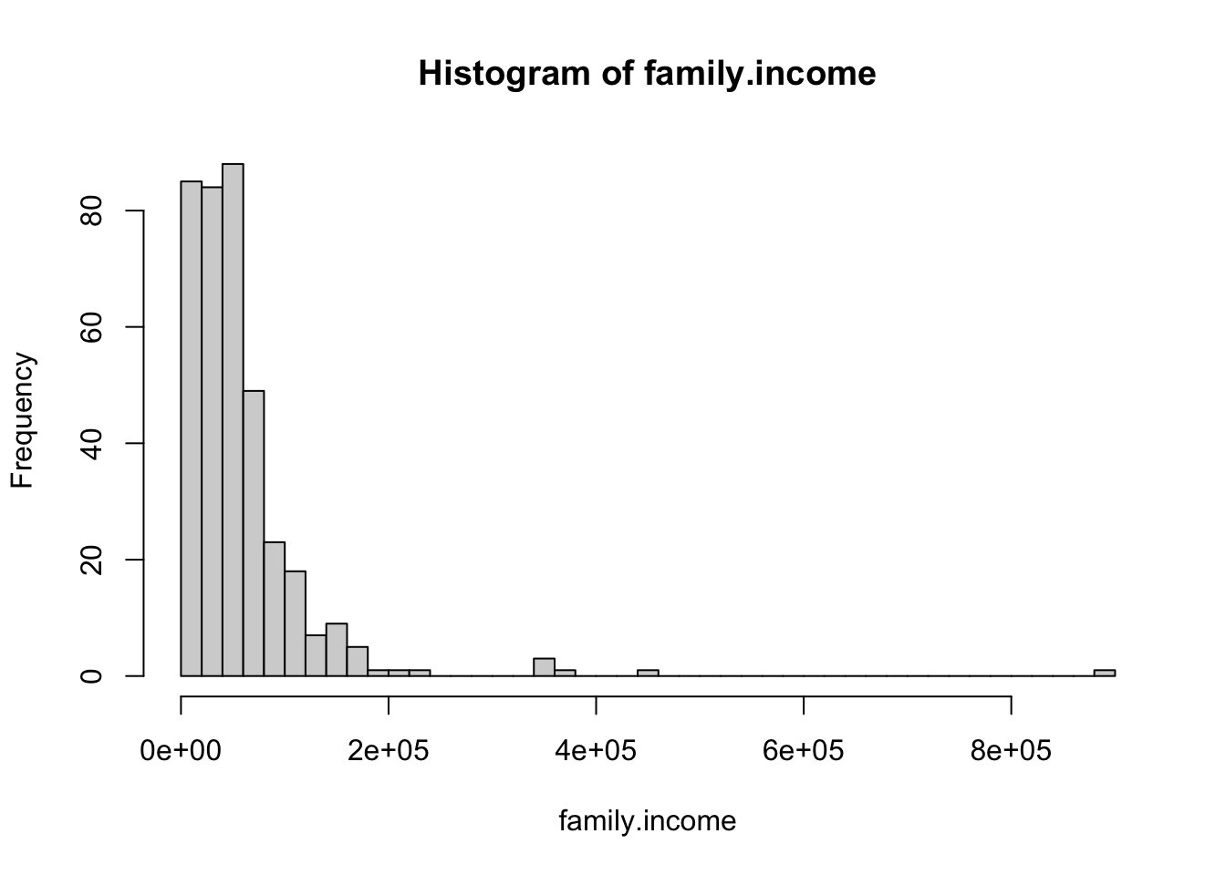
construct a histogram of total family incomes with an appropriate amount of binning
determine an appropriate measure of center
determine an appropriate measure of spread and interpret it in context
Solution
# load and inspect datasetload('data/census.RData')head(census)
  census_year state_fips_code total_family_income age    sex    race_general
1        2000         Florida               14550  44   Male Two major races
2        2000         Florida               22800  20 Female           White
3        2000         Florida                   0  20   Male           Black
4        2000         Florida               48000  55   Male           White
5        2000         Florida               74000  43 Female           White
6        2000         Florida               23000  60 Female           White
          marital_status total_personal_income
1 Married/spouse present                     0
2   Never married/single                 13000
3   Never married/single                 20000
4 Married/spouse present                 36000
5 Married/spouse present                 27000
6 Married/spouse present                 11800
There are 8 columns in the dataframe, so not including year and FIPS, there are 6 variables.
Not including FIPS, there are 3 categorical variables: sex, race_general, and marital_status
There are 377 individuals in the sample (one per row).
# part d: minimum and maximum ageage <- census$agemin(age)
[1] 15
max(age)
[1] 93
# part e: histogram of family incomesfamily.income <- census$total_family_incomehist(family.income, breaks =50)
# part f: measure of centermedian(family.income)
[1] 44000
# part g: measure of spreadIQR(family.income)
[1] 48000
The incomes are heavily right-skewed with some large outliers, so median and IQR are better choices of summary statistics.
Interpretation of IQR: the middle 50% of incomes are within 48K of one another.
The cdc.samp dataset in the oibiostat package contains a sample of data for 60 individuals surveyed by the CDC’s Behavioral Risk Factors Surveillance System (BRFSS). Use the provided commands to load the dataset and then inspect it the usual way. Notice that several of the variables are 1’s and 0’s. Use the provided command ?oibiostat::cdc.samp to view the data documentation.
What do the values (1’s and 0’s) mean in the exerany variable?
What proportion of the sample are men? What proportion are women?
For each general health category, find the proportion of respondents who rated themselves in that category.
How many of the respondents have health coverage? (Hint:sum(x) will add up the values in a vector x; adding up a collection of 1’s and 0’s is equivalent to counting the number of 1’s.)
What percentage of the respondents have health coverage?
Solution
# load datadata('cdc.samp', package ='oibiostat')# check documentation?oibiostat::cdc.samp# part b: proportions of men and womensex <- cdc.samp$gendertable(sex) |>proportions()
sex
        m         f
0.4833333 0.5166667
# part c: proportions of respondents in each general health categoryhealth <- cdc.samp$genhlthtable(health) |>proportions()
health
 excellent  very good       good       fair       poor
0.28333333 0.30000000 0.28333333 0.11666667 0.01666667
# part d: number of respondents with health coveragecoverage <- cdc.samp$hlthplansum(coverage)
[1] 50
# part e: percentage of respondents with health coverage100*sum(coverage)/60