Homework 3

With solutions

Author

Your Name Here

Before you begin

Fill in the author and calpoly-id fields at the very top of this file. Replace "Your Name Here" with your full name and "yourpolynetid" with your Cal Poly username (the part of your email before @calpoly.edu, e.g. jdoe01). Your submission cannot be matched to your record without this.

Where a problem asks you to save a result by a specific name (shown in bold), use the exact name given — your work is checked automatically.

Refer to Lab 6 for problem 1, Lab 7 for problems 3 and 4, and Lab 8 for problems 5 and 6.

Question 1: Plant growth

The plantgrowth dataset includes measurements of dry weight of plants grown using one of two fertilizer treatments or no fertilizer (control); treatments were randomly allocated to plants.

library(tidyverse)
library(effectsize)
library(emmeans)
load('data/plantgrowth.RData')

Part a: Boxplots [L3]

Construct side-by-side boxplots of the data to assess ANOVA model assumptions.

Solution

boxplot(weight ~ group, data = plantgrowth)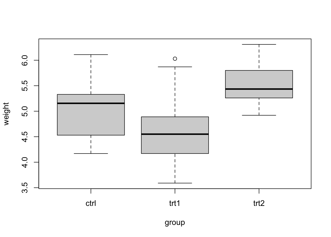

The distributions show similar variability, and individually \(t\) test assumptions seem plausible considering the small sample sizes – no severe skewness or extreme outliers.

Part b: Omnibus test [L9]

Fit an ANOVA model and test for a difference in mean dry weight among treatment groups at the 5% significance level. Report the result of the omnibus test in context following conventional style.

Solution

fit.plant <- aov(weight ~ group, data = plantgrowth)
summary(fit.plant)

            Df Sum Sq Mean Sq F value Pr(>F)  
group        2  3.766  1.8832   4.846 0.0159 *
Residuals   27 10.492  0.3886                 
---
Signif. codes:  0 '***' 0.001 '**' 0.01 '*' 0.05 '.' 0.1 ' ' 1

The data provide evidence that fertilizer treatment affects mean dry weight (F = 4.846 on 2 and 27 df, p = 0.0159).

Part c: Effect size [L9]

Estimate the effect size of fertilizer treatments on dry weight; provide a two-sided 95% confidence interval and interpret the interval in context.

Solution

eta_squared(fit.plant, alternative = 'two.sided')

# Effect Size for ANOVA

Parameter | Eta2 |       95% CI
-------------------------------
group     | 0.26 | [0.01, 0.49]

With 95% confidence, an estimated 1%-49% of variation in mean dry weight is attributable to fertilizer treatment.

Part d: Post-hoc comparisons [L9]

Test for significant differences in mean dry weight between each treatment compared with the control at the 5% level. Identify any significant differences.

Solution

emmeans(fit.plant, ~ group) |>
  contrast('trt.vs.ctrl') |>
  test(adjust = 'dunnett')

 contrast    estimate    SE df t.ratio p.value
 trt1 - ctrl   -0.371 0.279 27  -1.331  0.3296
 trt2 - ctrl    0.494 0.279 27   1.772  0.1582

P value adjustment: dunnettx method for 2 tests

Neither treatment differs significantly from the control.

Part e: Interpretation [L9]

How do you explain the apparent discrepancy between the omnibus test and the post-hoc comparisons?

Solution

The treatments differ significantly from each other, but not from the control.

Question 2: Longevity [Extra credit]

For the longevity study from lecture, follow the example to compute interval estimates for log-contrasts and back-transform interval endpoints to obtain estimates for the percent change in median lifespan relative to the control group. Report the comparison between the normal (N/N85) diet and the unrestricted (NP) diet. (Note: log(...) in R computes the natural logarithm \(\text{ln}(x)\) by default; the function exp(...) computes the exponential \(e^x\) by default; the two are inverses.)

load('data/longevity.RData')

Solution

# fit anova model to log lifetimes
fit.log <- aov(log(lifetime) ~ diet, data = longevity)

# estimate contrasts with control
emmeans(fit.log, ~ diet) |>
  contrast('trt.vs.ctrl') |>
  confint(level = 0.95, adjust = 'dunnett')

 contrast     estimate     SE  df lower.CL upper.CL
 (N/N85) - NP    0.200 0.0434 233   0.0972    0.303
 (N/R50) - NP    0.452 0.0413 233   0.3538    0.550
 (N/R40) - NP    0.524 0.0429 233   0.4217    0.625

Results are given on the log (not the response) scale. 
Confidence level used: 0.95 
Conf-level adjustment: dunnettx method for 3 estimates

# back-transform point estimate for n85/np contrast
exp(0.200)

[1] 1.221403

# back-transform interval estimates
c(exp(0.097), exp(0.303))

[1] 1.101860 1.353914

With 95% confidence, median lifespan is an estimated 10.2% and 35.4% longer among mice on an 85kCal diet relative to an unrestricted calorie diet.

Question 3: Cholesterol

The cholesterol dataset contains measurements of total serum cholesterol (mg/L) from a study in which participants were randomly allocated to one of two breakfast diets: corn flakes or oat bran.

load('data/cholesterol.RData')

Part a: Boxplots [L5]

Construct boxplots of serum cholesterol by diet group. Why might a nonparametric method be more appropriate than the \(t\) test to compare groups?

Solution

boxplot(chol ~ diet, data = cholesterol, horizontal = T)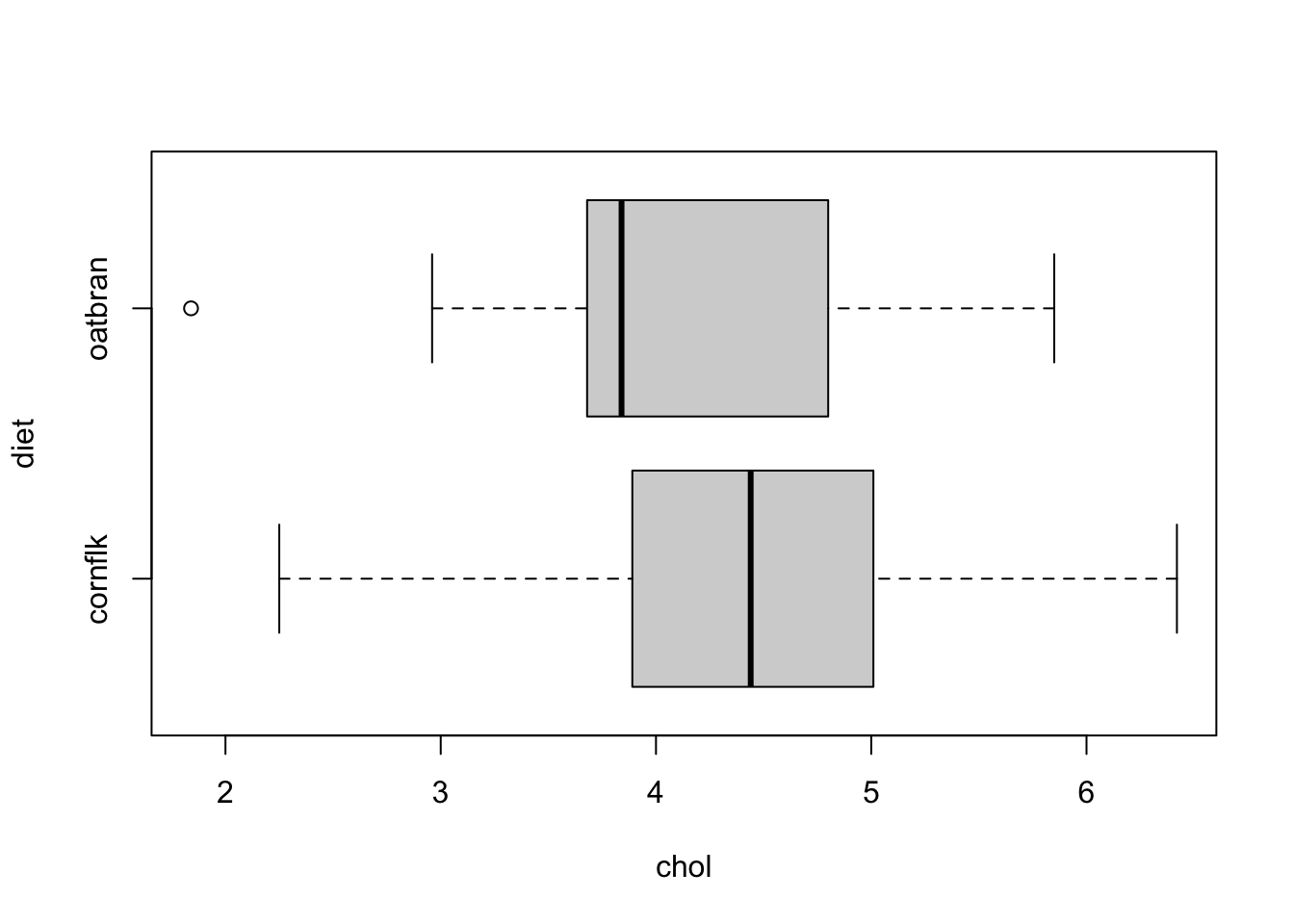

The distribution of cholesterol values in the oat bran group is right-skewed and includes an outlier.

Part b: Rank sum test [L5]

Test for an effect of diet on cholesterol using the rank sum procedure at the 5% level and interpret the result in context.

Solution

wilcox.test(chol ~ diet, data = cholesterol)


    Wilcoxon rank sum exact test

data:  chol by diet
W = 126, p-value = 0.2056
alternative hypothesis: true location shift is not equal to 0

The data do not provide evidence of an effect of diet on serum cholesterol (rank sum test, p = 0.2063).

Part c: Parametric comparison [L5]

Compare your results above with a parametric test. Do your conclusions differ depending on which procedure is used?

Solution

t.test(chol ~ diet, data = cholesterol)


    Welch Two Sample t-test

data:  chol by diet
t = 0.9469, df = 25.805, p-value = 0.3525
alternative hypothesis: true difference in means between group cornflk and group oatbran is not equal to 0
95 percent confidence interval:
 -0.4251218  1.1508361
sample estimates:
mean in group cornflk mean in group oatbran 
             4.443571              4.080714

The results differ minimally when the parametric test is used: the test conclusion is the same, and the estimated difference in means is of similar magnitude (0.36 vs. 0.40). However, the estimated difference is less precise using the parametric method (CI is wider).

Question 4: FAMUSS genotype

The famuss dataset contains measurements of percent change in dominant and nondominant arm strength after resistance training for 595 study participants, along with ACTN3 genotype, which is thought to be associated with muscle growth.

load('data/famuss.RData')

Part a: Boxplots [L9]

Construct boxplots of change in nondominant arm strength by genotype. Why might a nonparametric approach be preferable to ANOVA in this circumstance?

Solution

boxplot(ndrm.ch ~ genotype, data = famuss, horizontal = T)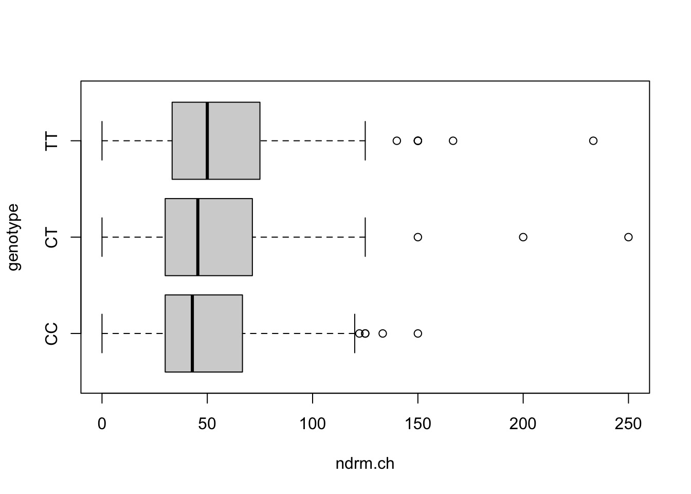

The data have many outliers; this does not conform to ANOVA assumptions.

Part b: Kruskal-Wallis test [L9]

Test for an association between genotype and change in nondominant arm strength at the 5% level using the Kruskal-Wallis test. Store the p-value as kw.famuss.pval. Interpret the result in context.

Solution

kw.famuss.pval <- kruskal.test(ndrm.ch ~ genotype, data = famuss)$p.value
kw.famuss.pval

[1] 0.05653417

The data do not provide evidence of an association between genotype and change in nondominant arm strength after resistance training (Kruskal-Wallis test, p = 0.0565).

Part c: Parametric comparison [L9]

Compare your result in the previous part with the parametric inference using ANOVA. Do conclusions differ?

Solution

aov(ndrm.ch ~ genotype, data = famuss) |> summary()

             Df Sum Sq Mean Sq F value Pr(>F)  
genotype      2   7043    3522   3.231 0.0402 *
Residuals   592 645293    1090                 
---
Signif. codes:  0 '***' 0.001 '**' 0.01 '*' 0.05 '.' 0.1 ' ' 1

The omnibus test for parametric ANOVA produces the opposite conclusion: the data provide evidence of an association (p = 0.0402).

Question 5: Crab claws

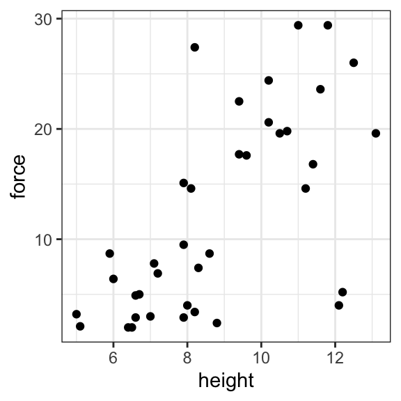
A study of the effects of predatory intertidal crab species on snail populations includes observations of propodus heights (mm) and closing strengths (Newtons) of the claws of crabs of three species. We will ignore species differences for this problem. A scatterplot of the data is shown below, along with the correlation coefficient and variable means.

height.mean	height.sd	force.mean	force.sd	corr
8.813	2.226	12.13	8.979	0.6533

Part a: Trend description [L10]

Describe the strength and direction of linear trend (if any).

Solution

The data show a moderate positive linear trend.

Part b: Least squares line [L10]

Compute the slope and intercept of the least squares line.

Solution

You can perform the calculation in R; the cell below provides space for this. However, you can also do the calculations on paper.

# summary statistics
r <- 0.6533
xbar <- 8.813
sx <- 2.226
ybar <- 12.13
sy <- 8.979

# slope estimate
beta1.hat <- r*sy/sx

# intercept estimate
beta0.hat <- ybar - beta1.hat*xbar

# print
c(slope = beta1.hat, intercept = beta0.hat)

     slope  intercept 
  2.635211 -11.094119

The slope and intercept for the least squares line are \(\hat{\beta}_1 = 2.635\) and \(\hat{\beta}_0 = -11.094\) respectively.

Part c: Slope interpretation [L10]

Interpret the slope coefficient in context.

Solution

With each 1-mm increase in propodus height, mean closing strength increases by 2.635 Newtons.

Question 6: Doctors and infant mortality

The doctors dataset contains observations of the number of doctors and the infant mortality rate (infant deaths per 1000 live births) in each of the 50 U.S. states in 2010.

load('data/doctors.RData')

Part a: Scatterplot [L10]

Based on the correlation coefficient and the scatterplot of the data, describe the apparent linear trend between number of doctors in a state and infant mortality (if any).

Solution

cor(doctors$doctors, doctors$inf.mort)

[1] -0.3267658

The correlation coefficient suggests a weak negative linear trend.

Part b: Linear model [L10]

Fit a linear model to the data, and plot the least squares line atop a scatterplot of the data.

Solution

fit <- lm(inf.mort ~ doctors, data = doctors)
plot(doctors$doctors, doctors$inf.mort,
     xlab = 'number of doctors', 
     ylab = 'infant mortality')
abline(coef = coef(fit), col = 'blue')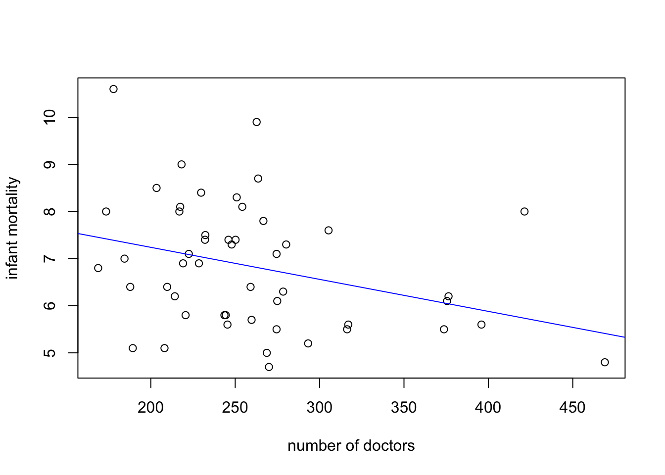

The plot is shown above.

Part c: Test for association [L10]

Do the data provide evidence of an association between infant mortality and the number of doctors at the 5% level? If so, what share of variation in infant mortality is explained by the number of doctors in a state?

Solution

summary(fit)


Call:
lm(formula = inf.mort ~ doctors, data = doctors)

Residuals:
    Min      1Q  Median      3Q     Max 
-2.2124 -0.9380 -0.1779  0.8077  3.2101 

Coefficients:
             Estimate Std. Error t value Pr(>|t|)    
(Intercept)  8.599061   0.760333  11.310 3.87e-15 ***
doctors     -0.006797   0.002837  -2.395   0.0206 *  
---
Signif. codes:  0 '***' 0.001 '**' 0.01 '*' 0.05 '.' 0.1 ' ' 1

Residual standard error: 1.278 on 48 degrees of freedom
Multiple R-squared:  0.1068,    Adjusted R-squared:  0.08817 
F-statistic: 5.738 on 1 and 48 DF,  p-value: 0.02055

The data provide evidence of an association between mean infant mortality rate and the number of doctors (T = -2.395 on 48 df, p = 0.0206). However, the number of doctors in a state only explains an estimated 10% of variation in infant mortality.

Part d: Confidence interval for trend [L10]

Construct and interpret a 95% confidence interval for the estimated change in infant mortality rate associated with adding 100 doctors to a state.

Solution

confint(fit)*100

                 2.5 %       97.5 %
(Intercept) 707.030794 1012.7813332
doctors      -1.250198   -0.1091745

With 95% confidence, an increase of 100 doctors in a state is associated with an estimated decrease in infant mortality between 0.11 and 1.25 deaths per 1000 live births.

Part e: Prediction [L10]

Predict the infant mortality rate for a state with 250 doctors. Provide and interpret an appropriate interval estimate.

Solution

predict(fit, newdata = data.frame(doctors = 250), interval = 'prediction')

       fit      lwr     upr
1 6.899845 4.303199 9.49649

With 95% confidence, infant mortality for a state with 250 doctors is predicted to be between 4.30 and 9.50 deaths per 1000 live births.

Submitting this assignment

Save the file (Ctrl+S / Cmd+S).
Render to PDF: click Render or press Ctrl+Shift+K / Cmd+Shift+K.
Download both files: in the Files panel, check the .qmd and PDF, then click More ▾ → Export….
Upload the PDF to the Gradescope assignment for this homework.
Upload the .qmd file through the submission link on the course page.