Homework 5

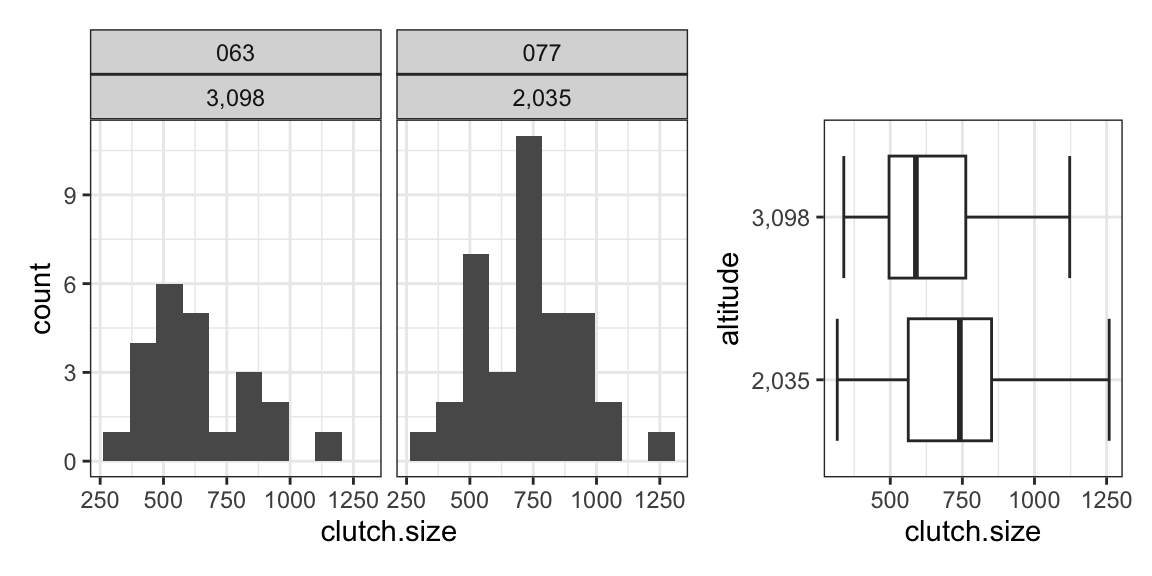
1. The table and figures below show summary statistics and distributions of clutch sizes for two of the sites in the frog data from Test 1.

   1. Compute a point estimate and standard error for the difference in mean clutch sizes between the two sites.
   2. Compute the test statistic you would use to test whether mean clutch size differs by site.
   3. Construct an approximate 99% confidence interval for the difference in mean clutch sizes.
   4. What would the conclusion of the test be at the 1% level?

site	altitude	csize.mean	csize.sd	n
063	3,098	625.67	197.01	23
077	2,035	733.44	202.72	37

Solution

# perform t test
test.out <- frog |>
  filter(site %in% c('077', '063')) |>
  select(site, altitude, clutch.size) %>%
  t.test(clutch.size ~ site, data = .)

# point estimate and std error
c(diff(test.out$estimate), test.out$stderr)

mean in group 077                   
        107.77512          52.89777 

# test statistic
test.out$statistic

        t 
-2.037423 

# 99.7% interval
diff(test.out$estimate) + c(-3, 3)*test.out$stderr

[1] -50.9182 266.4684

At the 1% level, there is no evidence of a difference in mean clutch size between frog populations at the two sites.

2. The lizards data contains top running speeds in meters per second (m/s) from two species of lizard: western fence and sagebrush.

   1. Construct side-by-side boxplots and comment on whether there appears to be a difference in mean top running speed between species. If so, which species appears to run faster?
   2. Test for a difference in mean top running speed between species at the 5% level. Report the test result following conventional style.
   3. Compute a point estimate for the difference in means and a standard error. Report the estimate following conventional style.
   4. Construct and interpret an interval estimate consistent with your test.

Solution

load('data/lizards.RData')

# side-by-side boxplots
boxplot(top.speed ~ species, data = lizards, horizontal = T)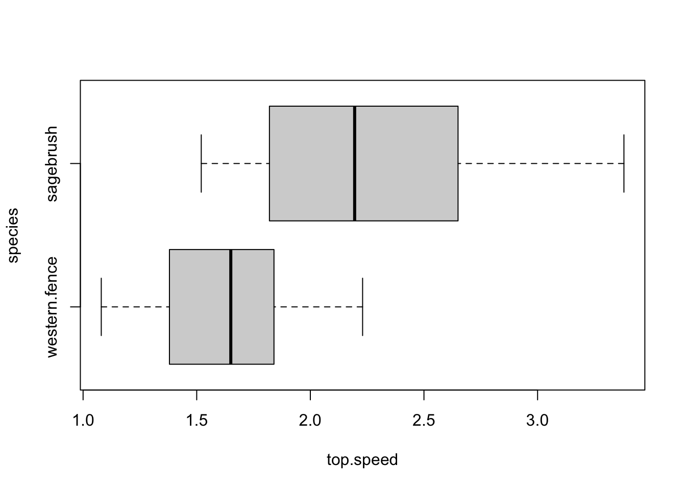

# test for a difference in mean top speed
tt.out <- t.test(top.speed ~ species, data = lizards)
tt.out

    Welch Two Sample t-test

data:  top.speed by species
t = -5.2217, df = 32.57, p-value = 9.939e-06
alternative hypothesis: true difference in means between group western.fence and group sagebrush is not equal to 0
95 percent confidence interval:
 -0.9754526 -0.4282537
sample estimates:
mean in group western.fence     mean in group sagebrush 
                   1.612692                    2.314545 

# point estimate and standard error
c(diff = diff(tt.out$estimate), se = tt.out$stderr)

diff.mean in group sagebrush                           se 
                   0.7018531                    0.1344115 

# confidence interval
tt.out$conf.int

[1] -0.9754526 -0.4282537
attr(,"conf.level")
[1] 0.95

1. Sagebrush lizards appear faster than western fence lizards.
2. The data provide evidence of a difference in mean top running speeds between western fence and sagebrush lizards (T = -5.2217 on 32.57 df, p < 0.0001).
3. The mean top running speed of sagebrush lizards is estimated to be 0.702 m/s faster than that of western fence lizards (SE 0.1344).
4. With 95% confidence, the mean top running speed of sagebrush lizards is estimated to be between 0.4283 and 0.9755 m/s faster than that of western fence lizards.