Homework 6

Course

STAT218

Due

May 6, 2025

library(tidyverse)
library(effectsize)
library(emmeans)

In a study¹, female mice were randomly assigned to four treatment groups to investigate whether restricting dietary intake increases life expectancy:

[NP] mice ate unlimited amount of nonpurified, standard diet
[N/N85] normal diet before weaning and normal diet after weaning (85 kcal/wk)
[N/R50] normal diet before weaning and reduced calorie diet after weaning (50 kcal/wk)
[N/R40] normal diet before weaning and reduced diet after weaning (40 Kcal/wk)

The longevity dataset contains observations of lifetime in weeks for 237 mice from the study described above. In this problem you’ll test whether diet restriction has an effect on longevity.
1. Make side-by-side boxplots of the lifespan data in each treatment group. Assess whether the model assumptions for ANOVA seem plausible.
2. Compute summary statistics by treatment group: sample means, standard deviations, sample sizes, and standard errors for the sample means.
3. Test for an effect of diet restriction on mean lifespan. Interpret the result of the test in context following the narrative format from class.
4. Estimate the effect size of diet restriction on mean lifespan; provide and interpret a (two-sided) 95% confidence interval.

Solution

# read in data and preview
load('data/longevity.RData')
head(longevity)

  lifetime diet
1     35.5   NP
2     35.4   NP
3     34.9   NP
4     34.8   NP
5     33.8   NP
6     33.5   NP

# part a: side-by-side boxplots
boxplot(lifetime ~ diet, data = longevity)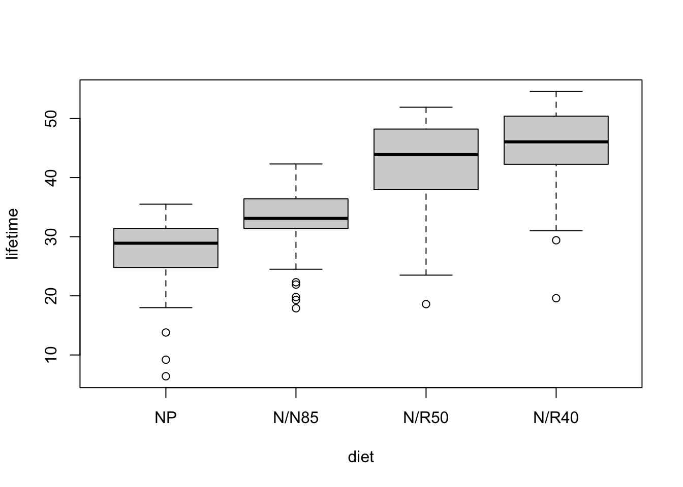

# part b: summary statistics by treatment group
longevity |>
  group_by(diet) |>
  summarize(mean = mean(lifetime),
            sd = sd(lifetime),
            n = length(lifetime),
            se = sd/sqrt(n))

# A tibble: 4 × 5
  diet   mean    sd     n    se
  <fct> <dbl> <dbl> <int> <dbl>
1 NP     27.4  6.13    49 0.876
2 N/N85  32.7  5.13    57 0.679
3 N/R50  42.3  7.77    71 0.922
4 N/R40  45.1  6.70    60 0.865

# part c: omnibus test for effect of diet on mean lifespan
fit <- aov(lifetime ~ diet, data = longevity)
summary(fit)

             Df Sum Sq Mean Sq F value Pr(>F)    
diet          3  11426    3809   87.41 <2e-16 ***
Residuals   233  10152      44                   
---
Signif. codes:  0 '***' 0.001 '**' 0.01 '*' 0.05 '.' 0.1 ' ' 1

# part d: estimate effect size
eta_squared(fit, partial = F, alternative = 'two.sided', ci = 0.95)

# Effect Size for ANOVA (Type I)

Parameter | Eta2 |       95% CI
-------------------------------
diet      | 0.53 | [0.44, 0.60]

The distributions show similar variability across groups, and individually data within groups satisfies $t$ test assumptions.
The data provide evidence that caloric intake affects mean lifespan (F = 87.41 on 3 and 233 df, p < 0.0001).
With 95% confidence, an estimated 44-60% of variation in lifespans is attributable to caloric intake.

Imagine you are designing a follow up study on dietary restriction.
1. If there are the same number of levels of dietary restriction as in the original study, how many mice per group would you need to detect an effect size of $η^{2} = 0.2$ 80% of the time using a 5% level test?
2. If there are only two levels of dietary restriction, and you want to detect a difference in mean lifespan of 1 week or more 90% of the time using a 5% level test, how many mice do you need in your study? (Round the largest standard deviation from the original study to the next nearest whole number for a conservative estimate.)
3. If there are six levels of dietary restriction, how many mice per group would you need to detect an effet of the same magnitude as estimated in the original study 85% of the time with a 5% level test?

Solution

# part a: same number of levels, effect size 0.2
power.anova.test(groups = 4,
                 sig.level = 0.05,
                 power = 0.8,
                 between.var = 0.2,
                 within.var = 0.8)


     Balanced one-way analysis of variance power calculation 

         groups = 4
              n = 15.54913
    between.var = 0.2
     within.var = 0.8
      sig.level = 0.05
          power = 0.8

NOTE: n is number in each group

# part b: two levels, difference of 1 week
power.t.test(delta = 7, 
             power = 0.9,
             sd = 8,
             sig.level = 0.05)


     Two-sample t test power calculation 

              n = 28.44356
          delta = 7
             sd = 8
      sig.level = 0.05
          power = 0.9
    alternative = two.sided

NOTE: n is number in *each* group

# part c: six levels, effect size same as in original study
power.anova.test(groups = 6,
                 sig.level = 0.05,
                 power = 0.85,
                 between.var = 0.53,
                 within.var = 0.47)


     Balanced one-way analysis of variance power calculation 

         groups = 6
              n = 3.602306
    between.var = 0.53
     within.var = 0.47
      sig.level = 0.05
          power = 0.85

NOTE: n is number in each group

[Extra credit] Continuing to refer to the longevity study above, follow the example from lecture to compute interval estimates for log-contrasts and back-transform interval endpoints to obtain estimates for the percent change in median lifespan relative to the control group. Report the comparison between the normal (N/N85) diet and the unrestricted (NP) diet. (Note: log(...) in R computes the natural logarithm $ln (x)$ by default; the function exp(...) computes the exponential $e^{x}$ by default; the two are inverses.)

Solution

load('data/longevity.RData')

# fit anova model to log lifetimes
fit.log <- aov(log(lifetime) ~ diet, data = longevity)

# estimate contrasts with control
emmeans(fit.log, ~ diet) |>
  contrast('trt.vs.ctrl') |>
  confint(level = 0.95, adjust = 'dunnett')

 contrast     estimate     SE  df lower.CL upper.CL
 (N/N85) - NP    0.200 0.0434 233   0.0972    0.303
 (N/R50) - NP    0.452 0.0413 233   0.3538    0.550
 (N/R40) - NP    0.524 0.0429 233   0.4217    0.625

Results are given on the log (not the response) scale. 
Confidence level used: 0.95 
Conf-level adjustment: dunnettx method for 3 estimates

# back-transform point estimate for n85/np contrast
exp(0.200)

[1] 1.221403

# back-transform interval estimates
c(exp(0.097), exp(0.303))

[1] 1.101860 1.353914

With 95% confidence, median lifespan is an estimated 10.2% and 35.4% longer among mice on an 85kCal diet relative to an unrestricted calorie diet.

The plantgrowth dataset includes measurements of dry weight of plants grown using one of two fertilizer treatments or no fertilizer (control); treatments were randomly allocated to plants.
1. Construct side-by-side boxplots of the data to assess ANOVA model assumptions.
2. Fit an ANOVA model and test for a difference in mean dry weight among treatment groups at the 5% significance level. Report the results in context following conventional style.
3. Estimate the effect size of fertilizer treatments on dry weight; provide a two-sided 95% confidence interval and interpret the interval in context.
4. Test for significant differences in mean dry weight between each treatment compared with the control at the 5% level. Identify any significant differences.
5. How do you explain the apparent discrepancy between the omnibus test and the post-hoc comparisons?

Solution

# load and inspect data
load('data/plantgrowth.RData')
head(plantgrowth)

  weight group
1   4.17  ctrl
2   5.58  ctrl
3   5.18  ctrl
4   6.11  ctrl
5   4.50  ctrl
6   4.61  ctrl

# construct side-by-side boxplots
boxplot(weight ~ group, data = plantgrowth)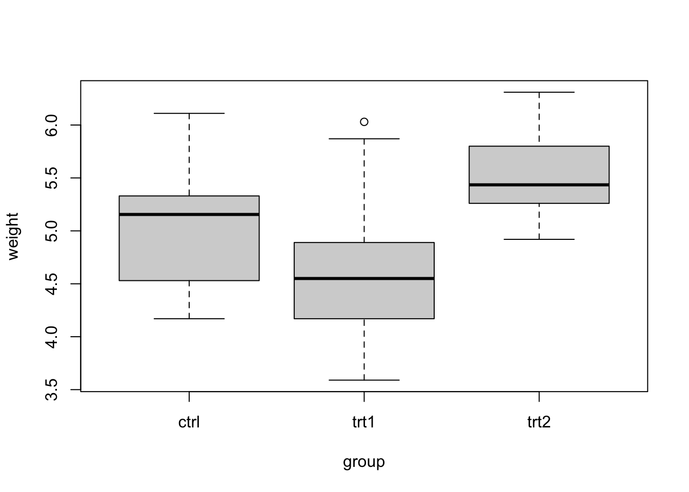

# fit anova model and perform omnibus test
fit.plant <- aov(weight ~ group, data = plantgrowth)
summary(fit.plant)

            Df Sum Sq Mean Sq F value Pr(>F)  
group        2  3.766  1.8832   4.846 0.0159 *
Residuals   27 10.492  0.3886                 
---
Signif. codes:  0 '***' 0.001 '**' 0.01 '*' 0.05 '.' 0.1 ' ' 1

# estimate effect size
eta_squared(fit.plant, alternative = 'two.sided')

# Effect Size for ANOVA

Parameter | Eta2 |       95% CI
-------------------------------
group     | 0.26 | [0.01, 0.49]

# test for contrasts with control
emmeans(fit.plant, ~ group) |>
  contrast('trt.vs.ctrl') |>
  test(adjust = 'dunnett')

 contrast    estimate    SE df t.ratio p.value
 trt1 - ctrl   -0.371 0.279 27  -1.331  0.3296
 trt2 - ctrl    0.494 0.279 27   1.772  0.1582

P value adjustment: dunnettx method for 2 tests

The distributions show similar variability, and individually $t$ test assumptions seem plausible considering the small sample sizes – no severe skewness or extreme outliers.
The data provide evidence that fertilizer treatment affects mean dry weight (F = 4.846 on 2 and 27 df, p = 0.0159).
With 95% confidence, an estimated 1%-49% of variation in mean dry weight is attributable to fertilizer treatment.
Neither treatment differs significantly from the control.
The treatments differ significantly from each other, but not from the control.

Footnotes

Weindruch, R., Walford, R.L., Fligiel, S. and Guthrie D. (1986). The Retardation of Aging in Mice by Dietary Restriction: Longevity, Cancer, Immunity and Lifetime Energy Intake, Journal of Nutrition 116(4):641–54.↩︎