Homework 7

library(tidyverse)
library(emmeans)
library(effectsize)

1. The plantgrowth dataset includes measurements of dry weight of plants grown using one of two fertilizer treatments or no fertilizer (control); treatments were randomly allocated to plants.

   1. Construct side-by-side boxplots of the data to assess ANOVA model assumptions.
   2. Fit an ANOVA model and test for a difference in mean dry weight among treatment groups at the 5% significance level. Report the results in context following conventional style.
   3. Estimate the effect size of fertilizer treatments on dry weight; provide a two-sided 95% confidence interval and interpret the interval in context.
   4. Test for significant differences in mean dry weight between each treatment compared with the control at the 5% level. Identify any significant differences.
   5. How do you explain the results of (c) in light of (d)?

Solution

# load and inspect data
load('data/plantgrowth.RData')
head(plantgrowth)

  weight group
1   4.17  ctrl
2   5.58  ctrl
3   5.18  ctrl
4   6.11  ctrl
5   4.50  ctrl
6   4.61  ctrl

# construct side-by-side boxplots
boxplot(weight ~ group, data = plantgrowth)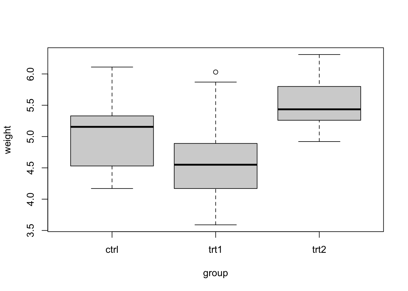

# fit anova model and perform omnibus test
fit.plant <- aov(weight ~ group, data = plantgrowth)
summary(fit.plant)

            Df Sum Sq Mean Sq F value Pr(>F)  
group        2  3.766  1.8832   4.846 0.0159 *
Residuals   27 10.492  0.3886                 
---
Signif. codes:  0 '***' 0.001 '**' 0.01 '*' 0.05 '.' 0.1 ' ' 1

# estimate effect size
eta_squared(fit.plant, alternative = 'two.sided')

# Effect Size for ANOVA

Parameter | Eta2 |       95% CI
-------------------------------
group     | 0.26 | [0.01, 0.49]

# test for contrasts with control
emmeans(fit.plant, ~ group) |>
  contrast('trt.vs.ctrl') |>
  test(adjust = 'dunnett')

 contrast    estimate    SE df t.ratio p.value
 trt1 - ctrl   -0.371 0.279 27  -1.331  0.3296
 trt2 - ctrl    0.494 0.279 27   1.772  0.1582

P value adjustment: dunnettx method for 2 tests 

1. The distributions show similar variability, and individually $t$ test assumptions seem plausible considering the small sample sizes – no severe skewness or extreme outliers.
2. The data provide evidence that fertilizer treatment affects mean dry weight (F = 4.846 on 2 and 27 df, p = 0.0159).
3. With 95% confidence, an estimated 1%-49% of variation in mean dry weight is attributable to fertilizer treatment.
4. Neither treatment differs significantly from the control.
5. The treatments differ significantly from each other, but not from the control.

2. [Extra credit] Using the longevity data from lecture, compute interval estimates for log-contrasts and back-transform to obtain estimates for the percent change in median lifespan relative to the control group. Report the comparison between the normal (N/N85) diet and the unrestricted (NP) diet.

Solution

load('data/longevity.RData')

# fit anova model to log lifetimes
fit.log <- aov(log(lifetime) ~ diet, data = longevity)

# estimate contrasts with control
emmeans(fit.log, ~ diet) |>
  contrast('trt.vs.ctrl') |>
  confint(level = 0.95, adjust = 'dunnett')

 contrast     estimate     SE  df lower.CL upper.CL
 (N/N85) - NP    0.200 0.0434 233   0.0972    0.303
 (N/R50) - NP    0.452 0.0413 233   0.3538    0.550
 (N/R40) - NP    0.524 0.0429 233   0.4217    0.625

Results are given on the log (not the response) scale. 
Confidence level used: 0.95 
Conf-level adjustment: dunnettx method for 3 estimates 

# back-transform point estimate for n85/np contrast
exp(0.200)

[1] 1.221403

# back-transform interval estimates
c(exp(0.0972), exp(0.303))

[1] 1.102081 1.353914

With 95% confidence, median lifespan is an estimated 10.2% and 35.4% longer among mice on an 85kCal diet relative to an unrestricted calorie diet.