Homework 8

1. The mammals data contain measurements of average brain weights (g) and average body weights (kg) for 62 mammal species. You will note that the ‘raw’ weights are stored as brain and body; log.brain and log.body record the log of the weights; and bb.ratio records the ratio of brain weight to body weight.

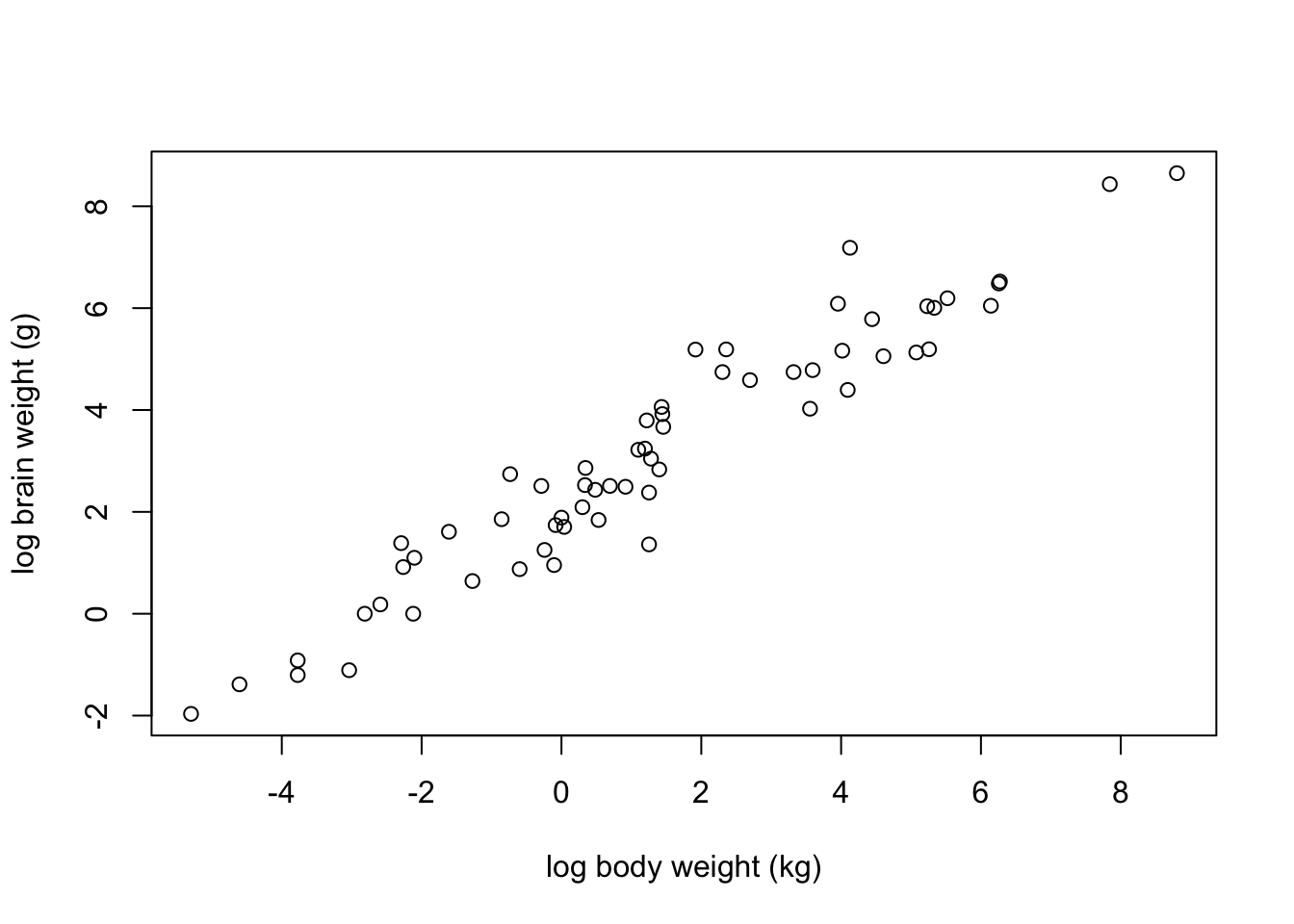
   1. [L3] Construct a scatterplot of log brain weight against log body weight with appropriate labels. (You should see a strong linear relationship; if not, you may have used the raw weights rather than the log-transformed weights.)
   2. [L3] Compute and interpret the correlation coefficient between log brain weight and log body weight. Your interpretation should note both the strength and direction of linear relationship between the variables.
   3. [L10] Compute the least squares estimates for a simple linear regression of log brain weight (response variable) on log body weight (explanatory variable). Interpret the slope coefficient in context.
   4. [L10] Estimate the proportion of variability explained by the model.

Solution

# load data
load('data/mammals.RData')

# plot log brain weight against log body weight
plot(log.brain ~ log.body, data = mammals, 
     xlab = 'log body weight (kg)', 
     ylab = 'log brain weight (g)')

# correlation between log brain weight and log body weight
cor(mammals$log.body, mammals$log.brain)

[1] 0.9595748

# least squares line
fit <- lm(log.brain ~ log.body, data = mammals)
fit

Call:
lm(formula = log.brain ~ log.body, data = mammals)

Coefficients:
(Intercept)     log.body  
     2.1348       0.7517  

2^0.7517

[1] 1.683776

# r squared
1 - 60*sigma(fit)^2/(61*var(mammals$log.brain))

[1] 0.9207837

1. The scatterplot is shown above; there is a clear linear trend.
2. The correlation indicates a strong positive linear relationship.
3. Every doubling of body weight is associated with a 68.38% increase in brain weight.
4. An estimated 92.1% of variation in (log) brain weight is explained by (log) body weight.

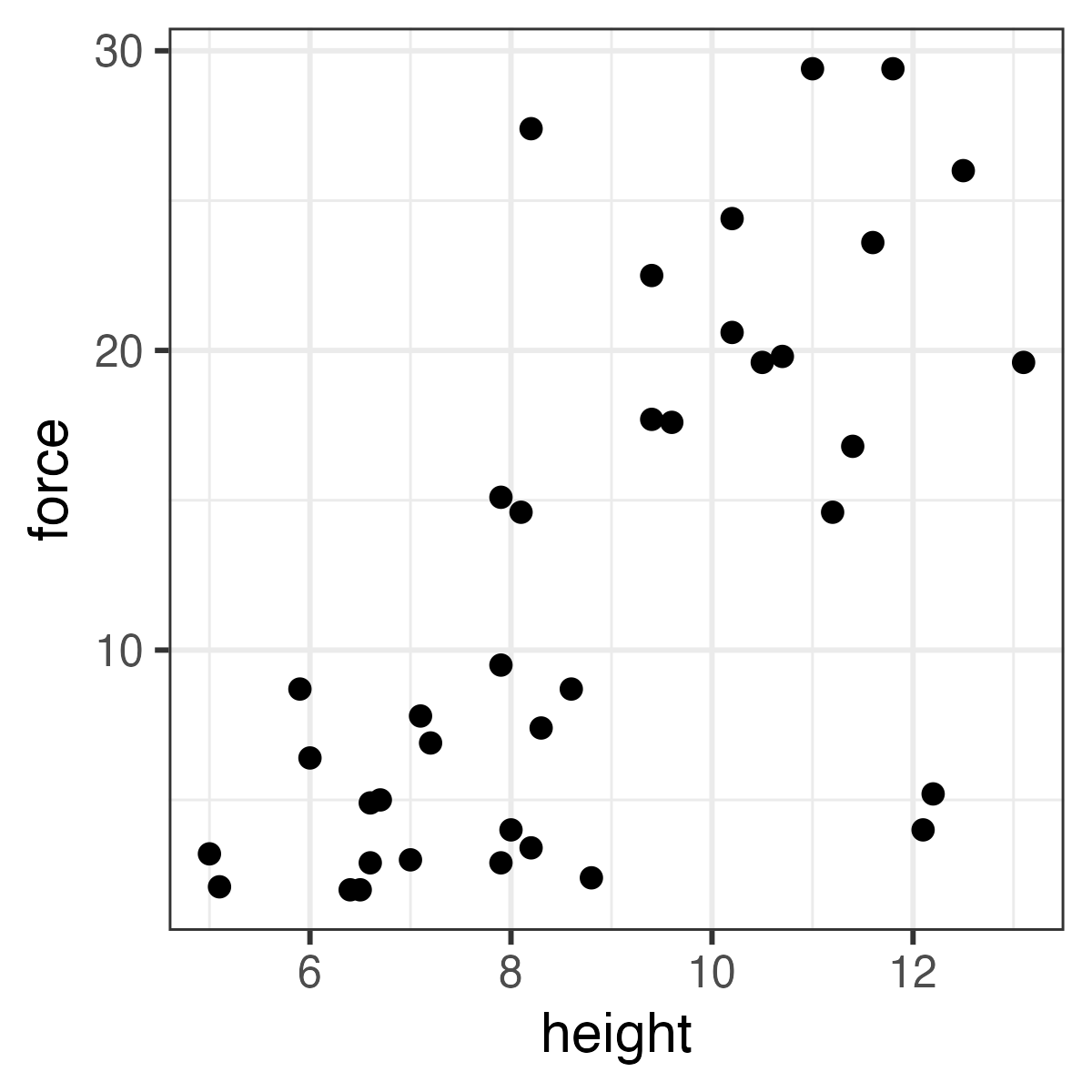
2. A study of the effects of predatory intertidal crab species on snail populations includes observations of propodus heights (mm) and closing strenths (Newtons) of the claws of crabs of three species. We will ignore species differences. A scatterplot of the data are shown below, along with the correlation coefficient and variable means.

   1. [L10] Describe the strength and direction of linear trend.
   2. [L10] Compute the slope and intercept of the least squares line.
   3. [L10] Interpret the slope coefficient in context.

height.mean	height.sd	force.mean	force.sd	corr
8.813	2.226	12.13	8.979	0.6533

Solution

You can perform the calculation in (b) in R; the cell below provides space for this. However, you can also do the calculations on paper.

# summary statistics
r <- 0.6533
xbar <- 8.813
sx <- 2.226
ybar <- 12.13
sy <- 8.979

# slope estimate
beta1.hat <- r*sy/sx

# intercept estimate
beta0.hat <- ybar - beta1.hat*xbar

# print
c(slope = beta1.hat, intercept = beta0.hat)

     slope  intercept 
  2.635211 -11.094119 

1. The data show a moderate positive linear trend.
2. The slope and intercept for the least squares line are given above.
3. With each 1-mm increase in propodus height, mean closing strength increases by 2.635 Newtons.