Homework 9

Course

STAT218

Due

May 20, 2025

library(tidyverse)
library(magrittr)
library(oibiostat)
load('data/frog.RData')
frog %<>% drop_na()
save(frog, file = 'data/frog2.RData')

data("census.2010")
doctors <- census.2010 |>
  filter(doctors < 800)
save(doctors, file = 'data/doctors.RData')

The frog2 dataset contains measurements of egg clutches collected from frogs populations at several sites in the Tibetan plateau. The variable clutch.size records the estimated number of eggs in the clutch, and the variable body.size records the length of the frog who laid the clutch in centimeters.
1. Plot clutch size against body size and describe the trend, if any. Be sure to include appropriate labels.
2. Compute and interpret the correlation between clutch size and body size.
3. Fit a simple linear regression model in which clutch size depends on body size. Write the estimated model equation.
4. Inspect the model summary. Do the data provide evidence of an association at the 5% level?
5. Construct and interpret a 95% confidence interval for the slope parameter.
6. Predict the mean clutch size among frogs 4.8cm in length. Provide an appropriate interval estimate.

Solution

# load data
load('data/frog2.RData')

# plot clutch size (y) against body size (x)
plot(frog$body.size, frog$clutch.size,
     xlab = "body size (cm)", ylab = "clutch size (# eggs)")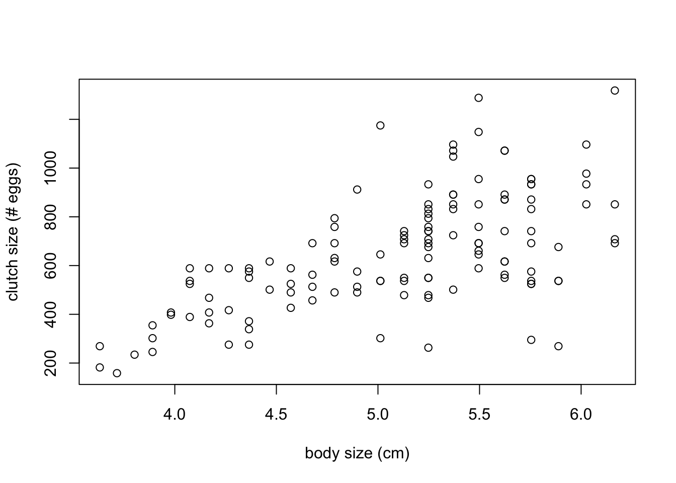

# compute correlation
cor(frog$body.size, frog$clutch.size)

[1] 0.6147564

# fit linear model
fit <- lm(clutch.size ~ body.size, data = frog)
fit


Call:
lm(formula = clutch.size ~ body.size, data = frog)

Coefficients:
(Intercept)    body.size  
     -507.2        227.6

# model summary
summary(fit)


Call:
lm(formula = clutch.size ~ body.size, data = frog)

Residuals:
    Min      1Q  Median      3Q     Max 
-563.96 -117.85   -0.87  112.90  544.59 

Coefficients:
            Estimate Std. Error t value Pr(>|t|)    
(Intercept)  -507.16     133.09  -3.811 0.000215 ***
body.size     227.61      25.91   8.784 9.21e-15 ***
---
Signif. codes:  0 '***' 0.001 '**' 0.01 '*' 0.05 '.' 0.1 ' ' 1

Residual standard error: 188 on 127 degrees of freedom
Multiple R-squared:  0.3779,    Adjusted R-squared:  0.373 
F-statistic: 77.16 on 1 and 127 DF,  p-value: 9.207e-15

# confidence interval for slope
confint(fit)

                2.5 %    97.5 %
(Intercept) -770.5326 -243.7967
body.size    176.3360  278.8891

# prediction for body length 4.8
predict(fit, 
        newdata = data.frame(body.size = 4.8),
        interval = 'confidence',
        level = 0.95)

       fit      lwr      upr
1 585.3758 549.2743 621.4773

There is a moderate positive linear trend between clutch size and body size.
The correlation is 0.6148.
The fitted model equation is $y = - 507.2 + 227.6 x$
The data provide evidence of an association between clutch size and body size (T = 8.78 on 127 df, p < 0.0001).
With 95% confidence, each 1cm increase in body length is associated with an estimated increase in clutch size between 176.34 and 278.89 eggs.
The predicted mean clutch size for a frog 4.8cm in length is 585.38 eggs. With 95% confidence, the mean clutch size for a frog 4.8cm in length is estimated to be between 549.27 and 621.48 eggs.

The doctors dataset contains observations of the number of doctors and the infant mortality rate (infant deaths per 1000 live births) in each of the 50 U.S. states in 2010.
1. Does there appear to be a linear trend between infant mortality and the number of doctors? Compute and interpret the correlation.
2. Fit a linear model to the data, and plot the least squares line atop a scatterplot of the data.
3. Do the data provide evidence of an association between infant mortality and the number of doctors at the 5% level?
4. Construct and interpret a 95% confidence interval for the linear trend: what is the estimated change in infant mortality rate associated with adding 100 doctors to a state?

Solution

# load data
load('data/doctors.RData')

# compute correlation
cor(doctors$doctors, doctors$inf.mort)

[1] -0.3267658

# fit linear model and plot atop data
fit <- lm(inf.mort ~ doctors, data = doctors)
plot(doctors$doctors, doctors$inf.mort,
     xlab = 'number of doctors', 
     ylab = 'infant mortality')
abline(coef = coef(fit), col = 'blue')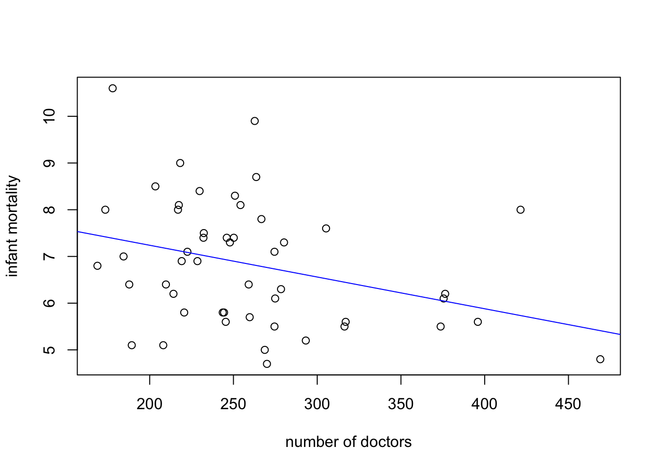

# test for an association
summary(fit)


Call:
lm(formula = inf.mort ~ doctors, data = doctors)

Residuals:
    Min      1Q  Median      3Q     Max 
-2.2124 -0.9380 -0.1779  0.8077  3.2101 

Coefficients:
             Estimate Std. Error t value Pr(>|t|)    
(Intercept)  8.599061   0.760333  11.310 3.87e-15 ***
doctors     -0.006797   0.002837  -2.395   0.0206 *  
---
Signif. codes:  0 '***' 0.001 '**' 0.01 '*' 0.05 '.' 0.1 ' ' 1

Residual standard error: 1.278 on 48 degrees of freedom
Multiple R-squared:  0.1068,    Adjusted R-squared:  0.08817 
F-statistic: 5.738 on 1 and 48 DF,  p-value: 0.02055

# interval estimate for trend
confint(fit)*100

                 2.5 %       97.5 %
(Intercept) 707.030794 1012.7813332
doctors      -1.250198   -0.1091745

The correlation coefficient suggests a weak negative linear trend.
The plot is shown above.
The data do provide evidence of an association between mean infant mortality rate and the number of doctors (T = -2.395 on 48 df, p = 0.0206).
With 95% confidence, an increase of 100 doctors in a state is associated with an estimated decrease in infant mortality between 0.11 and 1.25 deaths per 1000 live births.