Lab 11: Simple linear regression

Course activity

STAT218

The goal of this lab is to learn how to fit an SLR model, inspect the model summary, and generate confidence and prediction intervals. We’ll use the same datasets as last time.

load('data/prevend.RData')
load('data/mammals.RData')

Fitting an SLR model

To fit a linear model in R, use the lm(...) function:

# fit SLR model
fit.prevend <- lm(rfft ~ age, data = prevend)

The syntax here is y ~ x, which you can read as “y depends on x”. The names that you provide in the formula must match variable names in the dataset identified by the data = ... argument.

To print the least squares estimates of the model coefficients:

# print coefficient estimates
coef(fit.prevend)

(Intercept)         age 
 134.098052   -1.190794

Each additional year of age is associated with a 1.19-point decrease in mean RFFT score.

Your turn

Use lm(...) to fit a model to the mammal data relating log brain weight (y) to log body weight (x).

Store the model as fit.mammal. Print the coefficient estimates.

Solution

# fit SLR model
fit.mammal <- lm(log.brain ~ log.body, data = mammals)

# print coefficient estimates
coef(fit.mammal)

(Intercept)    log.body 
  2.1347887   0.7516859

Each 1-unit increment in log body weight is associated with a 0.75-unit increase in mean log brain weight.

If you wish to plot the fitted model over the data scatter, first make the plot and then add a line. (You have to run the whole cell for this to work.)

# visualize model
plot(prevend$age, prevend$rfft,
     xlab = 'age', ylab = 'RFFT score')
abline(coef = coef(fit.prevend), col = 'blue')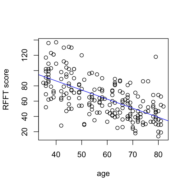

To obtain confidence intervals for the coefficients:

# confidence intervals for coefficients
confint(fit.prevend, level = 0.95)

                 2.5 %      97.5 %
(Intercept) 122.130647 146.0654574
age          -1.389341  -0.9922471

To see the model summary:

# model summary
summary(fit.prevend)


Call:
lm(formula = rfft ~ age, data = prevend)

Residuals:
    Min      1Q  Median      3Q     Max 
-56.085 -14.690  -2.937  12.744  77.975 

Coefficients:
            Estimate Std. Error t value Pr(>|t|)    
(Intercept) 134.0981     6.0701   22.09   <2e-16 ***
age          -1.1908     0.1007  -11.82   <2e-16 ***
---
Signif. codes:  0 '***' 0.001 '**' 0.01 '*' 0.05 '.' 0.1 ' ' 1

Residual standard error: 20.52 on 206 degrees of freedom
Multiple R-squared:  0.4043,    Adjusted R-squared:  0.4014 
F-statistic: 139.8 on 1 and 206 DF,  p-value: < 2.2e-16

The model summary shows several key pieces of information:

least squares estimates of coefficients and standard errors
significance tests of whether each model parameter is zero
estimated error variability $\hat{σ}$
proportion of variation explained by the model ( $R^{2}$ )

Take a moment to locate these.

Your turn

Print the model summary for your model of brain and body weights, and locate and interpret the relevant pieces of information listed above.

Solution

# model summary
summary(fit.mammal)


Call:
lm(formula = log.brain ~ log.body, data = mammals)

Residuals:
     Min       1Q   Median       3Q      Max 
-1.71550 -0.49228 -0.06162  0.43597  1.94829 

Coefficients:
            Estimate Std. Error t value Pr(>|t|)    
(Intercept)  2.13479    0.09604   22.23   <2e-16 ***
log.body     0.75169    0.02846   26.41   <2e-16 ***
---
Signif. codes:  0 '***' 0.001 '**' 0.01 '*' 0.05 '.' 0.1 ' ' 1

Residual standard error: 0.6943 on 60 degrees of freedom
Multiple R-squared:  0.9208,    Adjusted R-squared:  0.9195 
F-statistic: 697.4 on 1 and 60 DF,  p-value: < 2.2e-16

The estimates are ${\hat{β}}_{0} = 2.13479, {\hat{β}}_{1} = 0.75169, \hat{σ} = 0.6943$ .

The data provide evidence of an association between log body weight and log brain weight ( $T = 26.41$ on 60 df, $p < 0.0001$ ).

Log body weight explains an estimated 92.08% of log brain weight.

Predictions

To predict a new value for the response $y$ , the $x$ -value needs to be supplied in a particular format:

# predicted rfft score for a 55 year old
predict(fit.prevend, newdata = data.frame(age = 55))

       1 
68.60439

Your turn

A typical domestic cat weighs 3.5-4.5kg. Estimate its brain weight using your SLR model.

Does the estimate seem close? (Google “cat brain weight”.)

Solution

Replace the ....

# predicted log brain weight
pred <- predict(fit.mammal, 
                newdata = data.frame(log.body = log(4)))

# predicted brain weight in grams
exp(pred)

       1 
23.97105

According to google, the average brain weight of a domestic cat is 25-30g. The point estimate is a bit low compared to this value.

To add either a confidence or prediction interval, append additional arguments for the interval type and the desired coverage level:

# confidence interval for mean rfft score
predict(fit.prevend, newdata = data.frame(age = 55),
        interval = 'confidence', level = 0.95)

       fit     lwr      upr
1 68.60439 65.7101 71.49868

# prediction interval for specific rfft score
predict(fit.prevend, newdata = data.frame(age = 55),
        interval = 'prediction', level = 0.95)

       fit      lwr      upr
1 68.60439 28.04903 109.1598

Fit gives the point estimate, and lwr and upr give the left and right interval endpoints, respectively.

Recall that these two intervals have different interpretations. For the confidence interval:

With 95% confidence, the mean RFFT score among 55-year olds is estimated to be between 65.71 and 71.50 points.

Whereas for the prediction interval:

With 95% confidence, the predicted RFFT score for a 55-year-old individual is estimated to be between 28.05 and 109.16 points.

Your turn

Compute a confidence interval for your estimate from the last exercise. Does the interval capture the likely value?

Solution

Replace the ...

# predicted log brain weight
pred <- predict(fit.mammal, 
                newdata = data.frame(log.body = log(4)),
                interval = 'confidence')

# predicted brain weight in grams
exp(pred)

       fit      lwr     upr
1 23.97105 20.09453 28.5954

With 95% confidence, the brain weight of a typical 4kg domestic cat is estimated to be between 20.1 and 28.6 grams.

The confidence interval substantially overlaps with the range of 25-30 identified by internet search, so the estimate seems reasonable.

Now let’s have some fun with estimating brain weights.

Your turn

Estimate your brain weight by converting your body weight to kg and using the SLR model. Construct a prediction interval.

Then google “human brain weight”. Does the prediction seem reasonable? If not, can you speculate about why not?

Solution

Replace the ...

# predicted log brain weight
pred <- predict(fit.mammal, 
                newdata = data.frame(log.body = log(68)),
                interval = 'prediction')

# predicted brain weight in grams
exp(pred)

     fit      lwr      upr
1 201.65 49.25439 825.5651

The prediction interval is far too low. Biologically, humans have a larger-than-typical brain relative to their body mass.

If you’re interested, have a look at the animals sorted by decreasing brain-to-body ratio.

# arrange by descending bb ratio
dplyr::arrange(mammals, desc(bb.ratio))

                      mammal     body   brain    log.body  log.brain   bb.ratio
1            ground squirrel    0.101    4.00 -2.29263476  1.3862944 39.6039604
2                 owl monkey    0.480   15.50 -0.73396918  2.7408400 32.2916667
3  lesser short-tailed shrew    0.005    0.14 -5.29831737 -1.9661129 28.0000000
4              rhesus monkey    6.800  179.00  1.91692261  5.1873858 26.3235294
5                     galago    0.200    5.00 -1.60943791  1.6094379 25.0000000
6           little brown bat    0.010    0.25 -4.60517019 -1.3862944 25.0000000
7                   mole rat    0.122    3.00 -2.10373423  1.0986123 24.5901639
8                 tree shrew    0.104    2.50 -2.26336438  0.9162907 24.0384615
9                      human   62.000 1320.00  4.12713439  7.1853870 21.2903226
10                     mouse    0.023    0.40 -3.77226106 -0.9162907 17.3913043
11                    baboon   10.550  179.50  2.35612586  5.1901752 17.0142180
12           star-nosed mole    0.060    1.00 -2.81341072  0.0000000 16.6666667
13              rock hyrax-a    0.750   12.30 -0.28768207  2.5095993 16.4000000
14          e. american mole    0.075    1.20 -2.59026717  0.1823216 16.0000000
15                chinchilla    0.425    6.40 -0.85566611  1.8562980 15.0588235
16                    verbet    4.190   58.00  1.43270073  4.0604430 13.8424821
17                arctic fox    3.385   44.50  1.21935391  3.7954892 13.1462334
18             big brown bat    0.023    0.30 -3.77226106 -1.2039728 13.0434783
19                     genet    1.410   17.50  0.34358970  2.8622009 12.4113475
20                   red fox    4.235   50.40  1.44338333  3.9199912 11.9008264
21              patas monkey   10.000  115.00  2.30258509  4.7449321 11.5000000
22                   raccoon    4.288   39.20  1.45582042  3.6686767  9.1417910
23                slow loris    1.400   12.50  0.33647224  2.5257286  8.9285714
24                chimpanzee   52.160  440.00  3.95431592  6.0867747  8.4355828
25            golden hamster    0.120    1.00 -2.12026354  0.0000000  8.3333333
26                   echidna    3.000   25.00  1.09861229  3.2188758  8.3333333
27                       cat    3.300   25.60  1.19392247  3.2425924  7.7575758
28                 phalanger    1.620   11.40  0.48242615  2.4336134  7.0370370
29                musk shrew    0.048    0.33 -3.03655427 -1.1086626  6.8750000
30                       rat    0.280    1.90 -1.27296568  0.6418539  6.7857143
31                  roe deer   14.830   98.20  2.69665216  4.5870062  6.6217127
32 african giant pouched rat    1.000    6.60  0.00000000  1.8870696  6.6000000
33    arctic ground squirrel    0.920    5.70 -0.08338161  1.7404662  6.1956522
34                tree hyrax    2.000   12.30  0.69314718  2.5095993  6.1500000
35           mountain beaver    1.350    8.10  0.30010459  2.0918641  6.0000000
36              rock hyrax-b    3.600   21.00  1.28093385  3.0445224  5.8333333
37                guinea pig    1.040    5.50  0.03922071  1.7047481  5.2884615
38                    rabbit    2.500   12.10  0.91629073  2.4932055  4.8400000
39         european hedgehog    0.785    3.50 -0.24207156  1.2527630  4.4585987
40           desert hedgehog    0.550    2.40 -0.59783700  0.8754687  4.3636364
41     yellow-bellied marmot    4.050   17.00  1.39871688  2.8332133  4.1975309
42                      goat   27.660  115.00  3.31998733  4.7449321  4.1576283
43                 grey seal   85.000  325.00  4.44265126  5.7838252  3.8235294
44              n.a. opossum    1.700    6.30  0.53062825  1.8405496  3.7058824
45                 grey wolf   36.330  119.50  3.59264385  4.7833164  3.2892926
46                     sheep   55.500  175.00  4.01638302  5.1647860  3.1531532
47     nine-banded armadillo    3.500   10.80  1.25276297  2.3795461  3.0857143
48                    tenrec    0.900    2.60 -0.10536052  0.9555114  2.8888889
49                    donkey  187.100  419.00  5.23164323  6.0378709  2.2394441
50                   gorilla  207.000  406.00  5.33271879  6.0063532  1.9613527
51                     okapi  250.000  490.00  5.52146092  6.1944054  1.9600000
52            asian elephant 2547.000 4603.00  7.84267147  8.4344635  1.8072242
53                  kangaroo   35.000   56.00  3.55534806  4.0253517  1.6000000
54                    jaguar  100.000  157.00  4.60517019  5.0562458  1.5700000
55           giant armadillo   60.000   81.00  4.09434456  4.3944492  1.3500000
56                   giraffe  529.000  680.00  6.27098843  6.5220928  1.2854442
57                     horse  521.000  655.00  6.25575004  6.4846352  1.2571977
58             water opossum    3.500    3.90  1.25276297  1.3609766  1.1142857
59           brazilian tapir  160.000  169.00  5.07517382  5.1298987  1.0562500
60                       pig  192.000  180.00  5.25749537  5.1929569  0.9375000
61                       cow  465.000  423.00  6.14203741  6.0473722  0.9096774
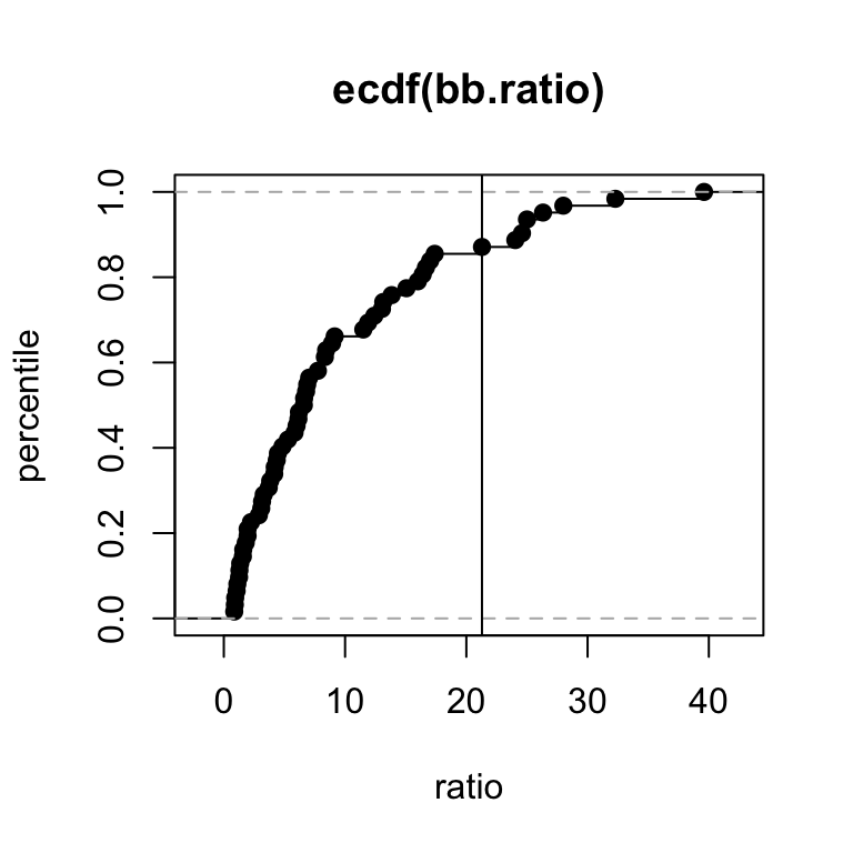
62          african elephant 6654.000 5712.00  8.80297346  8.6503245  0.8584310

The model might not predict as well at the extremes of the brain-to-body ratio. In particular, note below that humans are about at the 85th percentile.

# humans are at about the 85th percentile of brain-to-body ratios
bb.ratio <- mammals$bb.ratio
ecdf(bb.ratio) |> plot(xlab = 'ratio', ylab = 'percentile')
abline(v = bb.ratio[32])