Lab 8: Post-hoc inference in ANVOA

Course activity

STAT218

The objective of this lab is to learn how to perform post-hoc inference for group means and contrasts in R. These procedures are called post-hoc because they are typically performed after detecting a treatment effect or difference in means using the ANOVA $F$ test.

Examples will use the longevity and anorexia datasets, each of which is familiar by now. For the

library(tidyverse)
library(emmeans)
load('data/longevity.RData')
load('data/anorexia.RData')

Post-hoc inferences all utilize fitted ANOVA models. We will skip the step of making a graphical check on model assumptions, and proceed directly with fitting models.

# fit the model
fit.longevity <- aov(lifetime ~ diet, data = longevity)

# generate the ANOVA table
summary(fit.longevity)

             Df Sum Sq Mean Sq F value Pr(>F)    
diet          3  11426    3809   87.41 <2e-16 ***
Residuals   233  10152      44                   
---
Signif. codes:  0 '***' 0.001 '**' 0.01 '*' 0.05 '.' 0.1 ' ' 1

The ANOVA $F$ test is significant, indicating an effect of diet restriction on mean lifetime.

The data provide evidence of an effect of diet restriction on mean lifetime among mice (F = 87.41 on 3 & 233 degrees of freedom, p < 0.0001).

Your turn

Fit an ANOVA model to the anorexia data. Here, inference is on the mean percent change in body weight (the change variable in the dataset). Interpret the result of the test in context.

Solution

# fit the model
fit.anrx <- aov(change ~ treat, data = anorexia)

# generate the ANOVA table
summary(fit.anrx)

            Df Sum Sq Mean Sq F value Pr(>F)   
treat        2    615  307.32   5.422 0.0065 **
Residuals   69   3911   56.68                  
---
Signif. codes:  0 '***' 0.001 '**' 0.01 '*' 0.05 '.' 0.1 ' ' 1

The data provide evidence that therapy affects mean weight change (F = 5.422 on 2 and 69 df, p = 0.0065).

The emmeans(...) function (and other related functions) work directly with fitted ANOVA models to produce inferences for group means and contrasts. emmeans(...) is short for “estimated marginal means”. The function takes as its arguments a fitted ANOVA model, and a “specification” in the form of a formula that determines its precise behavior:

emmeans(object = <FITTED MODEL>, spec = <SPECIFICATION>)

For us, the specification is always a one-sided formula simply reiterating the grouping variable.

# basic emmeans call
emmeans(object = fit.longevity, specs = ~ diet)

 diet  emmean    SE  df lower.CL upper.CL
 NP      27.4 0.943 233     25.5     29.3
 N/N85   32.7 0.874 233     31.0     34.4
 N/R50   42.3 0.783 233     40.8     43.8
 N/R40   45.1 0.852 233     43.4     46.8

Confidence level used: 0.95

The default behavior of emmeans(...) is to produce estimated marginal means for each group and marginal (unadjusted) 95% confidence intervals. Compare this with the summary statistics:

# compare: emmeans uses a different standard error
longevity |>
  group_by(diet) |>
  summarize(mean = mean(lifetime),
            se = sd(lifetime)/sqrt(length(lifetime)))

# A tibble: 4 × 3
  diet   mean    se
  <fct> <dbl> <dbl>
1 NP     27.4 0.876
2 N/N85  32.7 0.679
3 N/R50  42.3 0.922
4 N/R40  45.1 0.865

You will recall from class that the standard error from the ANOVA model uses a pooled estimate of the population standard deviation. You can see this difference reflected above, though the difference is relatively small.

Your turn

Generate the estimated marginal means and marginal (unadjusted) confidence intervals for the model you fit to the anorexia data.

Solution

# estimated marginal means
emmeans(fit.anrx, specs = ~ treat)

 treat emmean   SE df lower.CL upper.CL
 ctrl   -0.45 1.48 69   -3.395      2.5
 cbt     3.01 1.40 69    0.218      5.8
 ft      7.26 1.83 69    3.622     10.9

Confidence level used: 0.95

Estimating group means

Initially we might like to estimate the group means. All we need to do is implement the adjustment for multiple inference and specify the confidence level. This is done using the confint(...) helper function:

# simultaneous 95% confidence intervals for group means with bonferroni adjustment (correct)
emmeans(object = fit.longevity, specs = ~ diet) |>
  confint(level = 0.95, adjust = 'bonferroni')

 diet  emmean    SE  df lower.CL upper.CL
 NP      27.4 0.943 233     25.0     29.8
 N/N85   32.7 0.874 233     30.5     34.9
 N/R50   42.3 0.783 233     40.3     44.3
 N/R40   45.1 0.852 233     43.0     47.3

Confidence level used: 0.95 
Conf-level adjustment: bonferroni method for 4 estimates

Take a moment to compare these results with the basic emmeans(...) call above. Note that the intervals are wider here to adjust for multiplicity, meaning that all four intervals cover the mean at the same time 95% of the time. As a result, we can interpret them together:

With 95% confidence, the mean lifetimes for mice on unrestricted, 85kcal, 50kCal, and 40cKal diets are estimated to be 25.0-29.8, 30.5-34.9, 40.3-44.3, and 43.0-47.3 days, respectively.

Your turn

Using the anorexia data, compute simultaneous 99% confidence intervals for the mean percent change in body weight in each treatment group and the control group. Interpret the interval for the family therapy (FT) group.

Solution

# simultaneous 99% confidence intervals for group means with bonferroni adjustment
emmeans(fit.anrx, ~ treat) |>
  confint(level = 0.99, adjust = 'bonferroni')

 treat emmean   SE df lower.CL upper.CL
 ctrl   -0.45 1.48 69    -4.94     4.04
 cbt     3.01 1.40 69    -1.24     7.26
 ft      7.26 1.83 69     1.71    12.82

Confidence level used: 0.99 
Conf-level adjustment: bonferroni method for 3 estimates

Sometimes a plot is preferable to a table of estimates. This is accomplished by adding one more pipe to plot(...) and specifying labels:

# plot via: emmeans(...) |> confint(...) |> plot(...)
emmeans(object = fit.longevity, specs = ~ diet) |> 
  confint(level = 0.95, adjust = 'bonferroni') |> 
  plot(xlab = 'mean lifetime (months)', ylab = 'diet')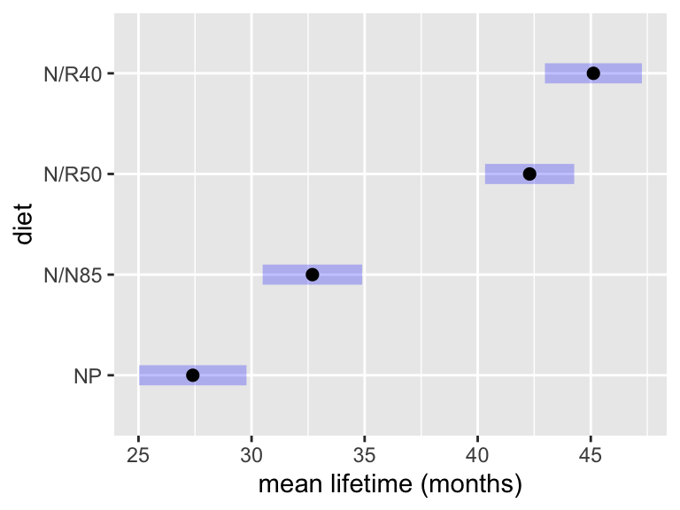

If you’re curious, remove the label arguments and see what the default looks like.

Your turn

Make a plot showing the simultaneous 99% interval estimates for the mean percent change in body weight that you computed in the previous “your turn”.

Solution

emmeans(fit.anrx, ~ treat) |>
  confint(level = 0.99, adjust = 'bonferroni') |>
  plot(xlab = 'mean weight change', ylab = 'therapy')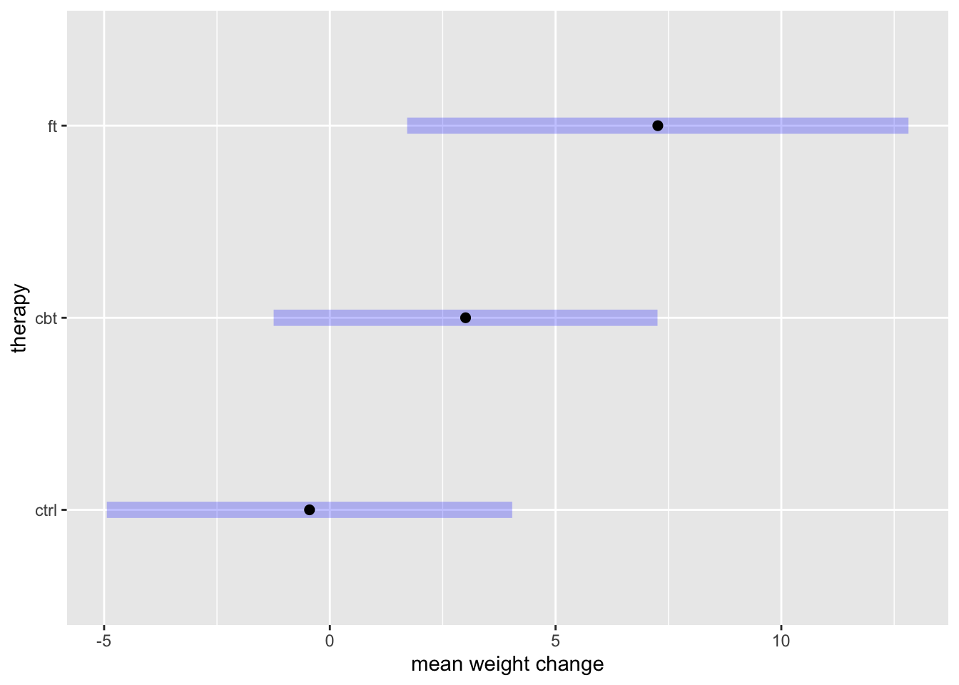

Estimating contrasts

In statistics, a difference in means is called a “contrast”. Inferences for contrasts allow us to determine which groups differ and by how much. There are several types of contrasts, but the most common are pairwise differences in means and differences between treatments and a control group.

Inference for pairwise contrasts

First we’ll consider computing intervals and tests for all pairwise contrasts. This is accomplished by simply passing the result of emmeans(...) to contrast(...) and specifying the type of contrast you wish to obtain.

# pairwise comparisons
emmeans(object = fit.longevity, specs = ~ diet) |>
  contrast('pairwise')

 contrast          estimate   SE  df t.ratio p.value
 NP - (N/N85)         -5.29 1.29 233  -4.113  0.0003
 NP - (N/R50)        -14.90 1.23 233 -12.150  <.0001
 NP - (N/R40)        -17.71 1.27 233 -13.938  <.0001
 (N/N85) - (N/R50)    -9.61 1.17 233  -8.183  <.0001
 (N/N85) - (N/R40)   -12.43 1.22 233 -10.177  <.0001
 (N/R50) - (N/R40)    -2.82 1.16 233  -2.436  0.0733

P value adjustment: tukey method for comparing a family of 4 estimates

By default this produces hypothesis tests of whether each contrast is zero. You may notice that the type of multiplicity adjustment is different (Tukey’s method rather than Bonferroni). If we want a different p-value adjustment, we can pass the result to test(...):

# tests with bonferroni correction
emmeans(object = fit.longevity, specs = ~ diet) |>
  contrast('pairwise') |>
  test(adjust = 'bonferroni')

 contrast          estimate   SE  df t.ratio p.value
 NP - (N/N85)         -5.29 1.29 233  -4.113  0.0003
 NP - (N/R50)        -14.90 1.23 233 -12.150  <.0001
 NP - (N/R40)        -17.71 1.27 233 -13.938  <.0001
 (N/N85) - (N/R50)    -9.61 1.17 233  -8.183  <.0001
 (N/N85) - (N/R40)   -12.43 1.22 233 -10.177  <.0001
 (N/R50) - (N/R40)    -2.82 1.16 233  -2.436  0.0937

P value adjustment: bonferroni method for 6 tests

If we want intervals, we can pass the result to confint():

# simultaneous 95% intervals
emmeans(object = fit.longevity, specs = ~ diet) |>
  contrast('pairwise') |>
  confint(level = 0.95, adjust = 'bonferroni')

 contrast          estimate   SE  df lower.CL upper.CL
 NP - (N/N85)         -5.29 1.29 233    -8.71   -1.867
 NP - (N/R50)        -14.90 1.23 233   -18.16  -11.633
 NP - (N/R40)        -17.71 1.27 233   -21.10  -14.333
 (N/N85) - (N/R50)    -9.61 1.17 233   -12.73   -6.482
 (N/N85) - (N/R40)   -12.43 1.22 233   -15.67   -9.177
 (N/R50) - (N/R40)    -2.82 1.16 233    -5.90    0.261

Confidence level used: 0.95 
Conf-level adjustment: bonferroni method for 6 estimates

The tests indicate which means differ significantly; the intervals indicate by how much. For example:

The data provide evidence that mean lifespan differs significantly between mice on a normal 85kcal compared with mice on an unrestricted diet (p = 0.0003). With 95% confidence, the difference in mean lifespan (normal - unrestricted) is estimated to be between 1.87 and 8.71 months, with a point estimate of 5.29 (SE 1.29).

It is conventional to check all pairwise contrasts, even if not all are reported; often, only significantly different contrasts are explicitly reported.

Your turn

Using the data from the anorexia study…

Compute simultaneous 90% confidence intervals for all pairwise contrasts.
Compute adjusted $p$ -values for all pairwise contrasts and determine which groups differ significantly at the 10% level.
Interpret the test and interval for the contrast between family therapy and the control group.

Solution

# simultaneous 90% intervals for all pairwise contrasts
emmeans(fit.anrx, ~treat) |>
  contrast('pairwise') |>
  confint(level = 0.9, adjust = 'bonferroni')

 contrast   estimate   SE df lower.CL upper.CL
 ctrl - cbt    -3.46 2.03 69    -7.87    0.958
 ctrl - ft     -7.71 2.35 69   -12.81   -2.616
 cbt - ft      -4.26 2.30 69    -9.25    0.736

Confidence level used: 0.9 
Conf-level adjustment: bonferroni method for 3 estimates

# test for pairwise differences at the 10% significance level
emmeans(fit.anrx, ~treat) |>
  contrast('pairwise') |>
  test(adjust = 'bonferroni')

 contrast   estimate   SE df t.ratio p.value
 ctrl - cbt    -3.46 2.03 69  -1.700  0.2808
 ctrl - ft     -7.71 2.35 69  -3.285  0.0048
 cbt - ft      -4.26 2.30 69  -1.852  0.2051

P value adjustment: bonferroni method for 3 tests

The data provide evidence that mean weight change differs between patients in family therapy and patients in the control group (T = -3.285 on 69 df, p = 0.0048); with 95% confidence, patients in family therapy are estimated to gain between 2.62 and 12.81 pounds more than patients in the control group.

Contrasts with a control

Many studies involve a control group; naturally, it is of interest to compare treatments to controls. This is a special category of contrasts because all contrasts involve the same group; as such, there is a special adjustment method for multiple inference that achieves better power for this particular setting.

To perform inference for contrasts with a control, change the contrast type from 'pairwise' to 'trt.vs.ctrl'. R will assume that your control group is the first level of the grouping variable. The datasets for this class are organized in just this way, so you don’t have to worry about this detail for now.

# tests for contrasts with a control group
emmeans(object = fit.longevity, specs = ~ diet) |>
  contrast('trt.vs.ctrl') |>
  test(adjust = 'dunnett')

 contrast     estimate   SE  df t.ratio p.value
 (N/N85) - NP     5.29 1.29 233   4.113  0.0002
 (N/R50) - NP    14.90 1.23 233  12.150  <.0001
 (N/R40) - NP    17.71 1.27 233  13.938  <.0001

P value adjustment: dunnettx method for 3 tests

# simultaneous 95% intervals for contrasts with a control group
emmeans(object = fit.longevity, specs = ~ diet) |>
  contrast('trt.vs.ctrl') |>
  confint(level = 0.95, adjust = 'dunnett')

 contrast     estimate   SE  df lower.CL upper.CL
 (N/N85) - NP     5.29 1.29 233     2.23     8.34
 (N/R50) - NP    14.90 1.23 233    11.98    17.81
 (N/R40) - NP    17.71 1.27 233    14.70    20.73

Confidence level used: 0.95 
Conf-level adjustment: dunnettx method for 3 estimates

The results indicate that all levels of diet restriction have an effect on mean lifetime that differs from the control group. Moreover, the intervals indicate that mean lifetimes are longer in every treatment group than in the control group; so diet restriction at every level causes an increase in lifetime.

Your turn

Using the data from the anorexia study…

Test, at the 1% significance level, for significant differences in mean percent change in body weight for each treatment compared with the control group. Are significant differences improvements relative to the control?
Estimate the efficacy (difference relative to control) of each treatment at the confidence level appropriate for the test you performed. Interpret the result in context.

Solution

# test for differences relative to control at 1% level
emmeans(fit.anrx, ~treat) |>
  contrast('trt.vs.ctrl') |>
  test(adjust = 'dunnett')

 contrast   estimate   SE df t.ratio p.value
 cbt - ctrl     3.46 2.03 69   1.700  0.1689
 ft - ctrl      7.71 2.35 69   3.285  0.0031

P value adjustment: dunnettx method for 2 tests

# estimate differences at the appropriate confidence level
emmeans(fit.anrx, ~treat) |>
  contrast('trt.vs.ctrl') |>
  confint(level = 0.99, adjust = 'dunnett')

 contrast   estimate   SE df lower.CL upper.CL
 cbt - ctrl     3.46 2.03 69   -2.420     9.33
 ft - ctrl      7.71 2.35 69    0.927    14.50

Confidence level used: 0.99 
Conf-level adjustment: dunnettx method for 2 estimates

Extra: testing a minimum difference

While not especially common, sometimes you might wish to test whether group means differ by at least a certain amount. The usual hypothesis tests for pairwise differences are: ${\begin{cases} H_{0} : & μ_{i} - μ_{j} = 0 \\ H_{A} : & μ_{i} - μ_{j} \neq 0 \end{cases}$ We could instead test for a minimum difference of $c$ by testing: ${\begin{cases} H_{0} : & | μ_{i} - μ_{j} | = c \\ H_{A} : & | μ_{i} - μ_{j} | > c \end{cases}$

This looks tricky on face value because of the absolute value. However, if the groups are ordered in R monotonically by means (i.e., in increasing/decreasing order of group mean), the signs for pairwise contrasts will all match, as they do in the example provided. In this case, the hypothesis above reduce, for $i > j$ , to: ${\begin{cases} H_{0} : & μ_{i} - μ_{j} = c \\ H_{A} : & μ_{i} - μ_{j} > c \end{cases}$

So, to test for a minimum difference, we simply do a directional test with a nonzero null value: add null = ... and side = ... arguments to test(...). In the context of comparisons with the control:

# test whether mean lifetime exceeds control by more than 2 weeks
emmeans(object = fit.longevity, specs = ~ diet) |>
  contrast('trt.vs.ctrl') |>
  test(null = 14, side = '>')

 contrast     estimate   SE  df null t.ratio p.value
 (N/N85) - NP     5.29 1.29 233   14  -6.774  1.0000
 (N/R50) - NP    14.90 1.23 233   14   0.730  0.5488
 (N/R40) - NP    17.71 1.27 233   14   2.923  0.0057

P value adjustment: sidak method for 3 tests 
P values are right-tailed

# interval estimate
emmeans(object = fit.longevity, specs = ~ diet) |>
  contrast('trt.vs.ctrl') |>
  confint(level = 0.95, side = '>')

 contrast     estimate   SE  df lower.CL upper.CL
 (N/N85) - NP     5.29 1.29 233     2.55      Inf
 (N/R50) - NP    14.90 1.23 233    12.28      Inf
 (N/R40) - NP    17.71 1.27 233    15.00      Inf

Confidence level used: 0.95 
Conf-level adjustment: sidak method for 3 estimates

Notice that a different adjustment method is used. This has a slightly more precise interpretation:

The data provide evidence that mean lifespan increases by at least two weeks when intake is restricted to 40kcal/day compared with an unrestricted diet (T = 2.923 on 233 degrees of freedom, p = 0.0057). With 95% confidence, the mean increase is estimated to be at least 15.00 days, with a point estimate of 17.71 days (SE 1.27).