load('data/census.RData')
load('data/temps.RData')
load('data/mussels.RData')Lab 9: nonparametric inference
The objective of this lab is to learn how to implement nonparamteric alternatives to
- sign test
- signed rank test
- rank sum test
- Kruskal-Wallis test
Examples utilize data from lecture and past assignments.
One-sample inference
Sign test
The sign test is a nonparametric inference procedure for inference on a population median
If the median is in fact
Here’s an example of testing whether median DDT in kale samples is 3:
# ddt data
ddt <- MASS::DDT

# how many observations are less than 3?
ddt.x <- sum(ddt < 3)
ddt.n <- length(ddt)

# sign test
binom.test(x = ddt.x, n = ddt.n, p = 0.5, alternative = 'two.sided')
    Exact binomial test

data:  ddt.x and ddt.n
number of successes = 2, number of trials = 15, p-value = 0.007385
alternative hypothesis: true probability of success is not equal to 0.5
95 percent confidence interval:
 0.01657591 0.40460270
sample estimates:
probability of success
             0.1333333
The
The data provide evidence that the median DDT in kale is not 3ppm (sign test, *p = 0.0074).
Your turn
Using the census data, test whether median total personal income is 25K using the sign test. Interpret the result in context.
Extra: Which alternative should you use in binom.test to test whether median income is less than 25K?
Solution
# incomes from census data
incomes <- census$total_personal_income

# how many observations are less than 25K?
incomes.x <- sum(incomes < 25000)
incomes.n <- length(incomes)

# sign test
binom.test(x = incomes.x, n = incomes.n, p = 0.5, alternative = 'two.sided')
    Exact binomial test

data:  incomes.x and incomes.n
number of successes = 228, number of trials = 377, p-value = 5.557e-05
alternative hypothesis: true probability of success is not equal to 0.5
95 percent confidence interval:
 0.5534322 0.6544581
sample estimates:
probability of success
             0.6047745
The data provide evidence that median income is not 25K.
Signed rank test
The signed rank test provides inference on the “center” of a population distribution, assuming the distribution is symmetric. For example, a two-sided test would pertain to the hypothesis and alternative:
Under the symmetry assumption, one can interpret the center as a median.
The implementation in R is almost identical to the wilcox.test(...). For example, to test whether median male body temperature is 98.7 degrees Farenheit:
# male body temperatures
temps.split <- split(temps$body.temp, temps$sex)
temps.m <- temps.split$male

# signed rank test
wilcox.test(temps.m, mu = 98.7, alternative = 'two.sided')
    Wilcoxon signed rank test with continuity correction

data:  temps.m
V = 39.5, p-value = 0.01505
alternative hypothesis: true location is not equal to 98.7
We’d interpret the result as follows:
The data provide evidence that median male body temperature is not 98.7 degrees Farenheit (signed rank test, p = 0.0151).
Your turn
Test whether median female body temperature is 98.7 degrees Farenheit and interpret the result in context.
Solution
# female body temperatures
temps.f <- temps.split$female

# signed rank test
wilcox.test(temps.f, mu = 98.7, alternative = 'two.sided')
    Wilcoxon signed rank test with continuity correction

data:  temps.f
V = 79, p-value = 0.7935
alternative hypothesis: true location is not equal to 98.7
The data do not provide evidence that median female body temperature differs from 98.7 degrees Farenheit.
It is important to remember that this method relies on assuming the underlying data distribution is symmetric.
Two-sample inference
Consider now comparing the centers of two groups. For this we can use the rank sum test, which for a two-sided alternative would assess the hypotheses:
This is the analogue of the two-sample
The implementation in R is straightforward. To test whether male and female body temperatures differ:
# rank sum test
wilcox.test(body.temp ~ sex, data = temps)
    Wilcoxon rank sum test with continuity correction

data:  body.temp by sex
W = 249.5, p-value = 0.09682
alternative hypothesis: true location shift is not equal to 0
We’d interpret the result as follows:
The data do not provide evidence that body temperatures differ by sex (rank sum test, p = 0.0968).
Your turn
Using the census data, test whether incomes are higher among men than among women. Interpret your result in context.
Solution
# rank sum test
wilcox.test(total_personal_income ~ sex, data = census, alternative = 'less')
    Wilcoxon rank sum test with continuity correction

data:  total_personal_income by sex
W = 11889, p-value = 1.363e-08
alternative hypothesis: true location shift is less than 0
The data provide evidence that incomes difer by sex (rank sum test, p < 0.0001).
By including conf.int and conf.level arguments, we can obtain an estimate and confidence interval for the magnitude of the location shift:
# rank sum test
wilcox.test(body.temp ~ sex, data = temps, conf.int = T, conf.level = 0.95)
    Wilcoxon rank sum test with continuity correction

data:  body.temp by sex
W = 249.5, p-value = 0.09682
alternative hypothesis: true location shift is not equal to 0
95 percent confidence interval:
 -0.1999996  1.1000358
sample estimates:
difference in location
             0.5000276
This is interpreted as follows:
Body temperatures are estimated to be 0.5 degrees Farenheit higher among women.
As discussed in lecture, the rank sum test is designed to detect differences in location – meaning that the alternative, though written in terms of centers, is really that the values from one group tend to be uniformly larger/smaller than those from the other group. It’s important to keep this in mind.
Kruskal-Wallis test
The Kruskal-Wallis test provides an alternative to ANOVA. The data on AAM length of mussels from five populations exhibited some large outliers in certain groups:
# aam lengths by location
boxplot(aam.length ~ location, data = mussels)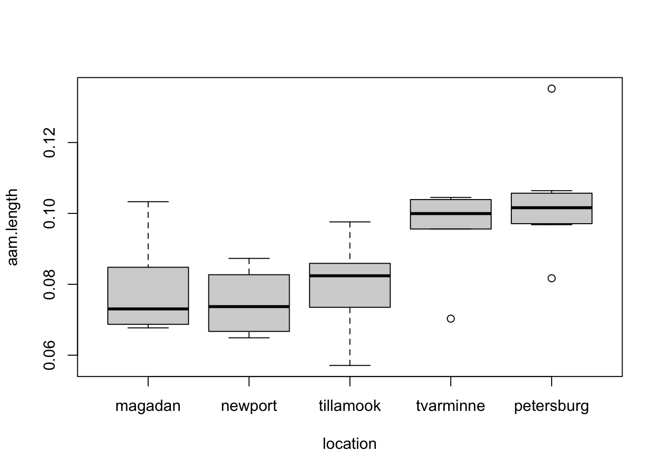
Owing to this feature, we might favor a rank-based alternative to the usual F test in ANOVA. This is implemented as follows:
# test for a difference in AAM length by location
kruskal.test(aam.length ~ location, data = mussels)
    Kruskal-Wallis rank sum test

data:  aam.length by location
Kruskal-Wallis chi-squared = 16.405, df = 4, p-value = 0.002521
Your turn
Using the census data, test whether personal incomes differ by race. Interpret your result in context.
Solution
# test for a difference in income distributions by race
kruskal.test(total_personal_income ~ race_general, data = census)
    Kruskal-Wallis rank sum test

data:  total_personal_income by race_general
Kruskal-Wallis chi-squared = 24.063, df = 7, p-value = 0.001111
The data provide evidence that personal income differs by race (Kruskal-Wallis test, p = 0.0011).
As an aside, note that the parametric test does not support the conclusion that incomes differ by race.
# compare with parametric alternative
aov(total_personal_income ~ race_general, data = census) |> summary()
Df Sum Sq Mean Sq F value Pr(>F)
race_general 7 2.960e+10 4.228e+09 1.967 0.0586 .
Residuals 369 7.933e+11 2.150e+09
---
Signif. codes: 0 '***' 0.001 '**' 0.01 '*' 0.05 '.' 0.1 ' ' 1The reason for this is that income distributions are right-skewed and heavy-tailed.
# boxplot of income distribution by race
par(mar = c(4, 15, 1, 1))
boxplot(total_personal_income ~ race_general, data = census,
        horizontal = T, las = 1, ylab = NULL)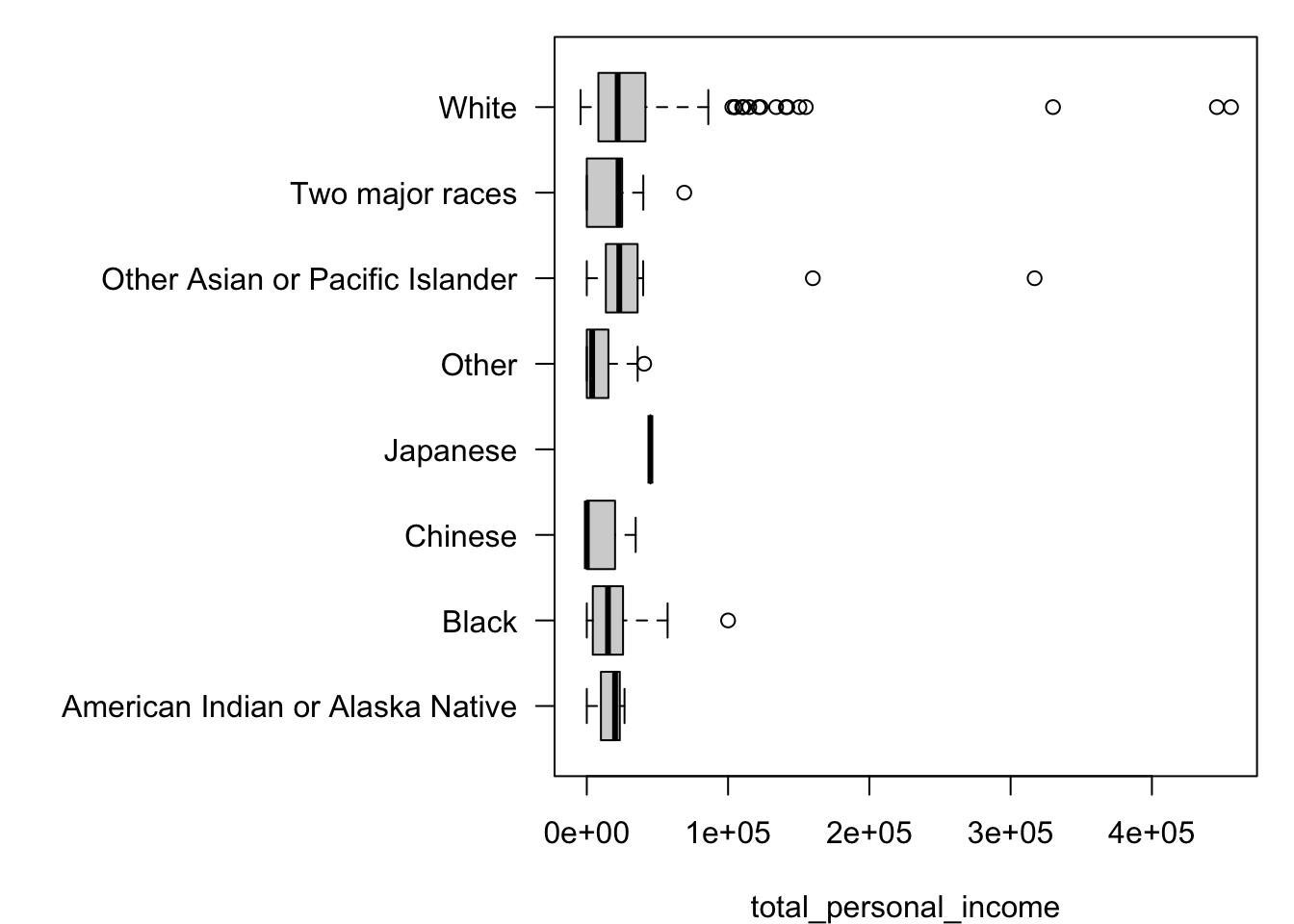
It’s worth noting that if this were a proper analysis, the racial groups would need to be recoded to address some issues in the current categorizations. For example, the data include only one individual identified as Japanese. For another example, it’s not clear how to interpret the biracial group in the analysis relative to the other categories, since they are presumably not mutually exclusive.