Here are some example questions representative of what you might see on the test.
[L2] Is this observational or experimental data?
[L1] Which variables are numeric and which are categorical?
[L1] Classify each numeric variable as discrete or continuous.
[L1] How many observations and variables are in the dataset?
[L3] What proportion of respondents are male?
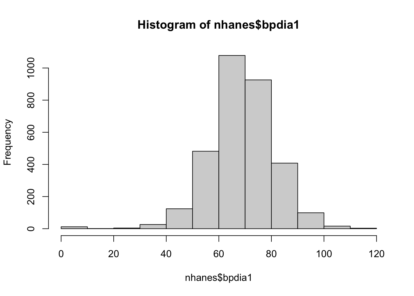
[L3] Make histograms of systolic and diastolic blood pressure (bpsys1 and bpdia1, respectively). Describe the distributions.
[L4] Construct 99% confidence intervals for mean systolic and diastolic blood pressure and interpret the intervals in context.
[L4] A person is considered to have hypertension if their systolic pressure is over 130 OR their diastolic pressure is over 80. Do the intervals suggest that the average adult has hypertension?
[L3] (challenge problem) How many individuals in the dataset have hypertension?
[L5] Test whether mean resting pulse is 72 bpm at the 5% level. Interpret the result of the test in context.
Solution
# proportion of male respondentstable(nhanes$gender) |>proportions()
   female      male
0.4995282 0.5004718
# histograms of systolic and diastolic blood pressurehist(nhanes$bpsys1)
hist(nhanes$bpdia1)
# intervals for systolic and diastolic blood pressure (quick way)t.test(nhanes$bpsys1, conf.level =0.99)
    One Sample t-test

data:  nhanes$bpsys1
t = 402.24, df = 3178, p-value < 2.2e-16
alternative hypothesis: true mean is not equal to 0
99 percent confidence interval:
 119.9750 121.5224
sample estimates:
mean of x
 120.7487
t.test(nhanes$bpdia1, conf.level =0.99)
    One Sample t-test

data:  nhanes$bpdia1
t = 314.42, df = 3178, p-value < 2.2e-16
alternative hypothesis: true mean is not equal to 0
99 percent confidence interval:
 69.01999 70.16088
sample estimates:
mean of x
 69.59044
# intervals for systolic and diastolic blood pressure (long way)bps.mean <-mean(nhanes$bpsys1)bps.se <-sd(nhanes$bpsys1)/sqrt(3179)cval <-qt(0.995, df =3178)bps.mean +c(-1, 1)*cval*bps.se
# how many individuals have hypertension (challenge)sys.over130 <- (nhanes$bpsys1 >130) dia.over80 <- (nhanes$bpdia1 >80)table(sys.over130 + dia.over80)
   0    1    2
2169  770  240
# test whether resting pulse is 72 bpmt.test(nhanes$pulse, mu =72, conf.level =0.95)
    One Sample t-test

data:  nhanes$pulse
t = 2.8235, df = 3178, p-value = 0.00478
alternative hypothesis: true mean is not equal to 72
95 percent confidence interval:
 72.18071 73.00205
sample estimates:
mean of x
 72.59138
Observational; this is survey data with no intervention.
All variables are numeric except for gender.
All variables are discrete (integer-valued) except for totchol.
There are 3179 observations of 8 variables.
50.05% of respondents were male.
Histograms are above; the distribution of systolic pressure is right-skewed, and the distribution of diastolic pressure is symmetric. Both are unimodal.
With 99% confidence, mean systolic pressure is estimated to be between 119.98 and 121.52 mmHg. With 99% confidence, mean diastolic pressure is estimated to be between 69.02 and 70.16 mmHg.
No: the intervals suggest neither mean is in the elevated range.
1010 individuals, or approximately one third of respondents, have hypertension.
The data provide evidence that mean resting pulse differs from 72 bpm (T = 2.82 on 3178 degrees of freedom, p = 0.00478).
Egg clutches
Data from Chen, W., et al., Maternal investment increases with altitude in a frog on the Tibetan Plateau. Journal of Evolutionary Biology 26-12 (2013) includes measurements pertaining to egg clutches of several populations of frog at breeding ponds (sites) in the eastern Tibetan Plateau. The first few rows are shown below.
One of the problems on the test uses this dataset. Use this space to explore the data and carry out possible summaries and analyses. You might practice one or more of the following:
descriptive statistics
graphical summaries (histograms, barplots)
point and interval estimates for a population mean