Test 2 practice (solutions)

Mussel physiology

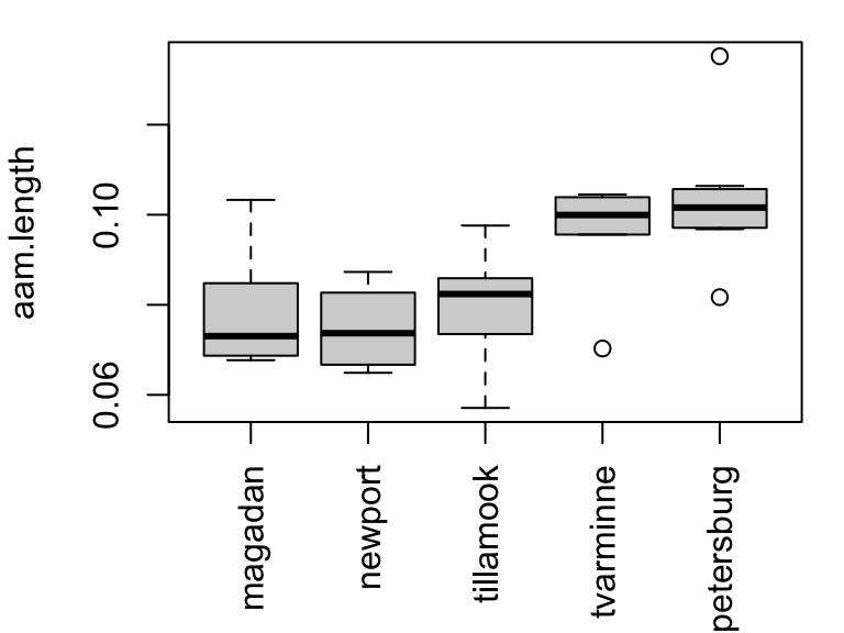
Researchers recorded observations of standardized anterior adductor muscle (AAM) scar length for mytilus trossulus mussels from five populations. The objective of the study was to identify physiological differences between populations. A plot of the data is provided below.

The output below shows an ANOVA model fitted to the data.

Call:
   aov(formula = aam.length ~ location, data = mussels)

Terms:
                   location   Residuals
Sum of Squares  0.004519674 0.005394906
Deg. of Freedom           4          34

Residual standard error: 0.01259658
Estimated effects may be unbalanced

1. [L9] How many mussels were measured in the study?

Solution

Since $34={\text{df}}_{\text{error}}=n-k$ and $4={\text{df}}_{\text{location}}=k-1$, the number of mussels is $n=34+4+1=39$.

2. [L9] Construct the ANOVA table.

Solution

The MS and F terms can be computed by hand from the SS and DF terms given above:

• $MS=\frac{SS}{df}$
• $F=\frac{M{S}_{\text{location}}}{M{S}_{\text{residuals}}}$

term	df	sumsq	meansq	statistic
location	4	0.00452	0.00113	7.121
Residuals	34	0.005395	0.0001587	NA

3. [L9] Report the outcome of the omnibus test following conventional style. (Assume a 5% level test.)

Solution

A 5% level test almost always rejects for $F>5$ (see “rules of thumb” from ANOVA lecture). From this you can conclude:

The data provide evidence that mean AAM length differs among mussel populations (F = 7.12 on 4 and 34 df).

4. [L9] Estimate the effect size ${\eta }^2$.

Solution

Recall ${\eta }^2=\frac{S{S}_{\text{location}}}{S{S}_{\text{location}}+S{S}_{\text{residual}}}$. This can be computed by hand from the output above.

0.00452/(0.00452 + 0.005395)

[1] 0.4558749

An estimated 46% of variation in AAM length is attributable to mussel population.

The output below shows pairwise comparisons for the five mussel populations.

 contrast               estimate      SE df t.ratio p.value
 magadan - newport       0.00321 0.00630 34   0.510  1.0000
 magadan - tillamook    -0.00219 0.00598 34  -0.366  1.0000
 magadan - tvarminne    -0.01769 0.00680 34  -2.600  0.1370
 magadan - petersburg   -0.02543 0.00652 34  -3.901  0.0043
 newport - tillamook    -0.00540 0.00598 34  -0.904  1.0000
 newport - tvarminne    -0.02090 0.00680 34  -3.072  0.0417
 newport - petersburg   -0.02864 0.00652 34  -4.394  0.0010
 tillamook - tvarminne  -0.01550 0.00650 34  -2.383  0.2291
 tillamook - petersburg -0.02324 0.00621 34  -3.744  0.0067
 tvarminne - petersburg -0.00774 0.00701 34  -1.105  1.0000

P value adjustment: bonferroni method for 10 tests 

5. [L9] Identify which populations have significantly different mean AAM lengths at the 1% level.

Solution

Three contrasts are significant at the 1% level (those with $p$ values under 0.01):

contrast	estimate	SE	df	t.ratio	p.value
magadan - petersburg	-0.02543	0.006519	34	-3.901	0.0043
newport - petersburg	-0.02864	0.006519	34	-4.394	0.001034
tillamook - petersburg	-0.02324	0.006208	34	-3.744	0.006696

The output below shows interval estimates for the mean AAM length of each population.

 location   emmean      SE df lower.CL upper.CL
 magadan    0.0780 0.00445 34   0.0659   0.0902
 newport    0.0748 0.00445 34   0.0626   0.0870
 tillamook  0.0802 0.00398 34   0.0693   0.0911
 tvarminne  0.0957 0.00514 34   0.0817   0.1097
 petersburg 0.1034 0.00476 34   0.0905   0.1164

Confidence level used: 0.95 
Conf-level adjustment: bonferroni method for 5 estimates 

6. [L4] Interpret the interval for the largest estimated mean AAM length in context.

Solution

With 95% confidence, mean standardized AAM length of Petersburg mussels is estimated to be between 0.0905 and 0.1164.

Creativity and motivation

This problem uses data from an experiment on the effect of intrinsic vs. extrinsic motivation on creativity. A random sample of 47 creative writing students at an unnamed university were randomly assigned to one of two groups. Each subject was instructed to write two short poems, but the instructions differed by group: one set of instructions alluded to external motivations for writing (e.g., recognition or reward), and the other alluded to internal motivations for writing (e.g., self-expression or personal satisfaction). Poems were scored by judges for creativity on a 40-point scale.

The output below shows a visualization of creativity scores by group, followed by inference on the difference in means.

    Welch Two Sample t-test

data:  score by treatment
t = -2.9153, df = 43.108, p-value = 0.005618
alternative hypothesis: true difference in means between group Extrinsic and group Intrinsic is not equal to 0
99 percent confidence interval:
 -7.9749541 -0.3134517
sample estimates:
mean in group Extrinsic mean in group Intrinsic 
               15.73913                19.88333 

1. [L5] Based on the boxplots, and the group sizes $n_{\text{intrinsic}}=24$ and $n_{\text{extrinsic}}=23$, do the assumptions for the inference shown seem plausible? Explain

Solution

The assumptions are that either the sample sizes are sufficiently large OR frequency distributions do not exhibit extreme outliers or extreme skewness for each group.

In this case, the distributions of creativity scores in each group are “well-behaved” – there are no outliers and there is no extreme skewness – so the assumptions for inference are plausible.

2. [L5] Write the hypothesis and alternative tested in statistical notation (i.e., in terms of ${\mu }_{\text{intrinsic}}$ and ${\mu }_{\text{extrinsic}}$).

Solution

The hypothesis and alternative are:

$$\begin{array}{r}{H}_0:{\mu }_{\text{extrinsic}}={\mu }_{\text{intrinsic}}\\ H_A:{\mu }_{\text{extrinsic}}\ne {\mu }_{\text{intrinsic}}\end{array}$$ Equivalently:

$$\begin{array}{r}{H}_0:{\mu }_{\text{extrinsic}}-{\mu }_{\text{intrinsic}}=0\\ H_A:{\mu }_{\text{extrinsic}}-{\mu }_{\text{intrinsic}}\ne 0\end{array}$$

3. [L5] Report the result of the 1% level test following conventional style.

Solution

The data provide evidence that mean writing creativity scores differ between extrinsically and intrinsically motivated students (T = -2.9153 on 43.1 df, p = 0.005618).

4. [L4] Interpret the confidence interval in context.

Solution

Either of the following is correct:

1. With 99% confidence, mean creativity scores are estimated to be between 0.31 and 7.97 points greater among intrinsically motivated students compared with extrinsically motivated students.

2. With 99% confidence, the difference in mean creativity scores between extrinsically and intrinsically motivated students is estimated to be between -7.97 and -0.31 points.

5. [L4] Construct a 95% confidence interval for the difference in means.

Solution

Since

$$T=\frac{{\overline{x}}_E-{\overline{x}}_I}{SE}$$

the standard error is

$$SE=\frac{{\overline{x}}_E-{\overline{x}}_I}{T}=\frac{15.73913-19.88333}{-2.9153}=1.4215$$

(15.73913 - 19.88333)/(-2.9153)

[1] 1.421535

# for comparison...
t.test(score ~ treatment, data = creativity, conf.level = 0.99)$stderr

[1] 1.42154

Once you get that, the 95% interval is just the point estimate plus/minus two standard errors:

(15.73913 - 19.88333) + c(-2, 2)*1.4215

[1] -6.9872 -1.3012

Hippocampal volume among schizophrenia patients

Studies have provided evidence that the hippocampus is smaller in schizophrenic patients on average. The dataset for this problem contains data on volumes of the left hippocampus in cubic centimeters for pairs of monozygotic twins; one twin in each pair was affected by schizophrenia and the other was not. The output below shows inference on the mean difference (affected - unaffected) in hippocampal volume between twins in each pair.

    One Sample t-test

data:  hvolume.diff
t = -3.2289, df = 14, p-value = 0.003031
alternative hypothesis: true mean is less than 0
99 percent confidence interval:
        -Inf -0.03718909
sample estimates:
 mean of x 
-0.1986667 

1. [L5] Write the hypothesis and alternative tested in statistical notation (i.e., in terms of the mean difference $\delta$).

Solution

The hypothesis and alternative are:

$$\begin{array}{r}{H}_0:\mu =0\\ H_A:\mu <0\end{array}$$

2. [L5] How many pairs of twins were included in the study?

Solution

Since $\text{df}=n-1$, there are $n=15$ pairs of twins in the study.

3. [L5] Report the result of the test following conventional style. (Use the level corresponding to the interval provided.)

Solution

The data provide evidence that mean volume of the left hippocampus is smaller among schizophrenic patients compared with their unaffected twins (T = -3.2289 on 14 df, p = 0.003031).

4. [L4] Interpret the confidence interval in context following conventional style.

Solution

With 99% confidence, the mean volume of the left hippocampus is estimated to be at least 0.037 cubic centimeters smaller among schizophrenic patients compared with their unaffected twins.

5. [L5] Compute the standard error of the point estimate for the mean difference in hippocampal volumes. Explain what this value quantifies.

Solution

Following the procedure from the last problem:

(-0.1986667)/(-3.2289)

[1] 0.06152767

This quantifies the average estimation error – on average, the estimated difference in hippocampal volume misses the population mean by 0.062 $c{m}^3$